Spatial Mixing of Coloring Random Graphs Yitong Yin Nanjing - PowerPoint PPT Presentation
Spatial Mixing of Coloring Random Graphs Yitong Yin Nanjing University Colorings undirected G(V,E) q colors: max-degree: d temporal mixing of Glauber dynamics approximately counting : 2 11/6 or sampling almost uniform proper q
Spatial Mixing of Coloring Random Graphs Yitong Yin Nanjing University
Colorings undirected G(V,E) q colors: max-degree: d temporal mixing of Glauber dynamics approximately counting α : 2 → 11/6 or sampling almost uniform proper q -colorings of G [Jerrum’95] [Vigoda’99] [Salas-Sokal’97] [Bubley-Dyer’97] when q ≥α d + β ? spatial mixing of Gibbs measure conjecture: α =1
Spatial Mixing undirected G(V,E) q colors: max-degree: d Gibbs measure: uniform random proper q -coloring of G c : V → [ q ] G region ∆ ⊇ ∂ R R ⊂ V ∆ proper q -colorings σ ∆ , τ ∆ : ∆ → [ q ] R t Pr[ c ( v ) = x | σ ∆ ] ≈ Pr[ c ( v ) = x | τ ∆ ] v error < exp (- t )
Spatial Mixing weak spatial mixing (WSM): Pr[ c ( v ) = x | σ ∆ ] ≈ Pr[ c ( v ) = x | τ ∆ ] strong spatial mixing (SSM): Pr[ c ( v ) = x | σ ∆ , σ Λ ] ≈ Pr[ c ( v ) = x | τ ∆ , σ Λ ] error < exp (- t ) G SSM: the value of ∆ critical to R Pr[ c ( v ) = x | σ Λ ] counting t and sampling v is approximable Λ by local information
Spatial Mixing of Coloring q -coloring of G q ≥α d +O( 1 ) max-degree: d average degree? SSM: α > 1.763... x x = e (solution to ) • [Goldberg, Martin, Paterson 05] triangle-free amenable graphs • [Ge, Stefankovic 11 ] regular tree • [Gamarnik, Katz, Misra 12 ] triangle-free graphs Spatial-mixing-based FPTAS: • [Gamarnik, Katz 07 ] α > 2.8432..., triangle-free graphs • Y. 14 ] α > 2.58071... [Lu, SSM ⇒ algorithm • [Goldberg, Martin, Paterson 05] amenable graph, SSM ⇒ FPRAS • [Y., Zhang 13 ] planar graph (apex-minor-free), SSM ⇒ FPTAS
Random Graph G ( n , d / n ) ✓ ln n average degree: d max-degree: whp ◆ Θ ln ln n q -colorable whp for a q =O( d /ln d ) rapid mixing of (block) Glauber dynamics: • [Dyer, Flaxman, Frieze, Vigoda 06] q =O(lnln n /lnlnln n ) • [Efthymiou, Spirakis 07] [Mossel, Sly 08] q =poly(d) • [Efthymiou 14 ] q >5.5 d + 1 spatial mixing?
Negative Result for SSM strong spatial mixing (SSM): for any vertex v Pr[ c ( v ) = x | σ ∆ , σ Λ ] ≈ Pr[ c ( v ) = x | τ ∆ , σ Λ ] for any q =O(1) in G( n , d / n ) G q colors: ∆ whp, ∃ : Ω (ln n ) long R t { } { } { } { } v Λ v u o q -2 This counter-example only affect the strong spatial mixing.
Main Result q ≥ α d + β for α >2 and some β =O(1) (23 is enough) fix any v ∈ [ n ] , and then sample G ( n , d / n ) whp : G ( n , d / n ) is q -colorable, and for any σ , τ | Pr[ c ( v ) = x | σ ] − Pr[ c ( v ) = x | τ ] | = exp ( − Ω ( t )) t = dist( v, ∆ ) = ω (1) G is the shortest distance ∆ from v to where σ , τ differ R t Strong Spatial Mixing v Λ w.r.t any fixed vertex!
Error Function error function [Gamarnik, Katz, Misra 12]: two distributions µ 1 , µ 2 : Ω → [0 , 1] ✓ ◆ log µ 1 ( x ) µ 2 ( x ) − log µ 1 ( y ) E ( µ 1 , µ 2 ) = max µ 2 ( y ) x,y ∈ Ω v ( x ) = Pr[ c ( v ) = x | σ ] and µ τ marginal distributions µ σ v E ( µ σ v ) ≤ exp( − Ω ( t )) v , µ τ | Pr[ c ( v ) = x | σ ] − Pr[ c ( v ) = x | τ ] | = exp ( − Ω ( t ))
Self-Avoiding Walk Tree G =( V , E ) T = T ��� ( G, v ) v
Error Propagation along Self-voiding Walks T = T ��� ( G, v ) 8 X v δ ( v i ) · E T i ,S v 62 S < E T,S = i v 3 v 1 3 q v 2 S v 2 : δ 0 δ ( 1 q > d ( u ) + 1 3 q q − d ( u ) − 1 3 q δ ( u ) = δ 3 q 1 o.w. S 0 3 q 1.0 δ 3 q S : permissive cut-set 0.9 0.8 • S separates ∆ from the root 0.7 • all u ∈ S and children: q > d ( u )+1 ∆ 0.6 • dist( S , ∆ ) ≥ 2 where σ , τ differ 0.5 d 0.4 1.0 1.5 2.0 2.5 3.0 3.5 4.0
Error Propagation along Self-voiding Walks T = T ��� ( G, v ) 8 X δ ( v i ) · E T i ,S v 62 S < E T,S = i 3 q v 2 S : δ 0 δ ( 1 q > d ( u ) + 1 3 q q − d ( u ) − 1 3 q δ ( u ) = δ 3 q 1 o.w. S 0 3 q 3 q S : permissive cut-set ∆ E ( µ σ v ) ≤ E T,S v , µ τ where σ , τ differ v : marginal distributions at v in G conditioning on σ , τ µ σ v , µ τ
Proof of Main Result v : marginal distributions at v in G conditioning on σ , τ µ σ v , µ τ ✓ ◆ v ( x ) v ( y ) log µ σ v ( x ) − log µ σ error function: E ( µ σ v ) = max v , µ τ v ( y ) µ τ µ τ x,y ∈ [ q ] S : permissive cut-set T = T ��� ( G, v ) correlation E ( µ σ v ) ≤ E T,S v , µ τ decay: for where G = G ( n , d / n ) T = T ��� ( G, v ) whp : always exists a permissive cut-set S probabilistic E T,S = exp( − Ω ( t )) method:
( 1 q > d ( u ) + 1 q − d ( u ) − 1 δ ( u ) = E ( µ σ v ) ≤ E T,S v , µ τ 1 o.w. T = T ��� ( G, v ) E T,S if v and all children have v for v ∈ S v 3 v 1 q > d ( u ) + 1 v 2 δ 0 δ then E ( µ σ v ) ≤ 3 q v , µ τ 3 q 3 q δ 3 q S 0 3 q 3 q if q > d ( u ) + 1 for all u 1 X E ( µ σ v , µ τ v ) ≤ q − d ( v i ) − 1 · E ( µ σ v i , µ τ v i ) ∆ i where defined in G \ { v } µ σ v i , µ τ v i (with altered color lists)
[Gamarnik, Katz, Misra 12 ]: 1 if q > d ( u ) + 1 for all u X E ( µ σ v , µ τ v ) ≤ q − d ( v i ) − 1 · E ( µ σ v i , µ τ v i ) i ✓ v ( x ) v ( y ) ◆ ✓ v ( x ) v ( x ) ◆ log µ σ v ( x ) − log µ σ log µ σ v ( y ) − log µ τ E ( µ σ v ) = max = max v , µ τ v ( y ) v ( y ) µ τ µ τ µ σ µ τ x,y ∈ Ω x,y ∈ Ω Pr( c ( v ) = y | σ ) = Pr G \{ v } ( 8 i, c ( v i ) 6 = x | σ ) v ( x ) v ( y ) = Pr( c ( v ) = x | σ ) where µ σ Pr G \{ v } ( 8 i, c ( v i ) 6 = y | σ ) µ σ 1 � Pr G \{ v } ( c ( v i ) = x | σ ) (telescopic product) Y = 1 � Pr G \{ v } ( c ( v i ) = y | σ ) i X X ⇥ � � � �⇤ ⇥ � � � �⇤ = log 1 − µ σ v i ( x ) − log 1 − µ τ v i ( x ) log 1 − µ σ v i ( y ) − log 1 − µ τ v i ( y ) − i i v i ( x ) v i ( y ) µ 0 log µ τ log µ τ (mean value theorem) µ i X X i = v i ( x ) − 1 − µ i 1 − µ 0 v i ( y ) µ σ µ σ i i i 1 where µ i , µ 0 i ≤ max { µ τ v i ( x ) , µ σ v i ( x ) , µ τ v i ( y ) , µ σ v i ( y ) } ≤ q − d ( v i ) 1 v i ( x ) v i ( y ) 1 ✓ log µ σ v i ( x ) − log µ σ ◆ X � � q − d ( v i ) − 1 E µ σ v i , µ τ X ≤ q − d ( v i ) − 1 max ≤ v i v i ( y ) µ τ µ τ x,y i i
For unbounded degree: q colors: when calculating correlation decay along path: { } available colors = end up with an infeasible coloring effectively × ∞ in calculating correlation decay: • error function [Gamarnik-Katz-Misra’12] • recursive coloring [Goldberg-Martin-Paterson’05] • computation tree [Gamarnik-Katz’07] • computation tree with potential function [Lu-Y.’14]
Block-wise Correlation Decay vertex v grows to a G permissive block B ∋ v q > d ( u ) + 1 ∀ u ∈ ∂ B, B v minimal permissive block B around v ∀ u ∈ B \ { v } , q ≤ d ( u ) + 1 B of colorings of B consider marginal distributions µ σ B , µ τ (averaging principle) E ( µ σ v ) ≤ E ( µ σ B ) v , µ τ B , µ τ (telescopic product + 1 X E ( µ σ B ) ≤ q − d ( v i ) − 1 · E ( µ σ v i ) B , µ τ v i , µ τ mean value theorem) i boundary vertices of B
( 1 q > d ( u ) + 1 q − d ( u ) − 1 δ ( u ) = E ( µ σ v ) ≤ E T,S v , µ τ 1 o.w. T = T ��� ( G, v ) for v E ( µ σ v ) ≤ 3 q v , µ τ v ∈ S G v 3 v 1 v 2 δ 0 δ ∆ 3 q 3 q v B δ 3 q S S 0 3 q 3 q E ( µ σ v ) ≤ E ( µ σ B ) v , µ τ B , µ τ ∆ 1 X q − d ( v i ) − 1 · E ( µ σ v i ) v i , µ τ ≤ i where are boundary vertices of B v i and defined in G \ B µ σ v i , µ τ v i
Random Self-Avoiding Walks for where G = G ( n , d / n ) T = T ��� ( G, v ) whp : always exists a permissive cut-set S whp E T,S = exp( − Ω ( t )) E [ E T,S ] = exp( − Ω ( t )) T = T ��� ( G, v ) is like a Galton-Watson random tree with binomial degree distribution B ( n -1, d / n ) each d ( u ) ∼ B ( n -1, d / n ) for when q > α d + O (1) α > 2 a permissive cut-set S of depth > t /2 exists 1 ( 1 q > d ( u ) + 1 E [ δ ( u )] < q − d ( u ) − 1 δ ( u ) = q − d 1 o.w.
Summary q ≥ α d + O(1) for α >2 • SSM for q -colorings of G ( n , d / n ) w.r.t. fixed vertex: • a block-wise decay of correlation for colorings of graphs with unbounded degree • Algorithmic implication is still open: • With SSM, local information is sufficient to estimate marginals. What local structure of G(n,d/n) can be exploited to efficiently compute marginals? • Path-coupling of block Glauber Dynamics replies on correlation decay.
Thank you! Any questions?
Recommend
More recommend
Explore More Topics
Stay informed with curated content and fresh updates.
