Sparse Johnson-Lindenstrauss Transforms Jelani Nelson MIT May 24, - PowerPoint PPT Presentation

Sparse Johnson-Lindenstrauss Transforms Jelani Nelson MIT May 24, 2011 joint work with Daniel Kane (Harvard)

Metric Johnson-Lindenstrauss lemma Metric JL (MJL) Lemma, 1984 Every set of n points in Euclidean space can be embedded into O ( ε − 2 log n )-dimensional Euclidean space so that all pairwise distances are preserved up to a 1 ± ε factor.

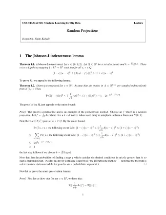
Metric Johnson-Lindenstrauss lemma Metric JL (MJL) Lemma, 1984 Every set of n points in Euclidean space can be embedded into O ( ε − 2 log n )-dimensional Euclidean space so that all pairwise distances are preserved up to a 1 ± ε factor. Uses: • Speed up geometric algorithms by first reducing dimension of input [Indyk-Motwani, 1998], [Indyk, 2001] • Low-memory streaming algorithms for linear algebra problems [Sarl´ os, 2006], [LWMRT, 2007], [Clarkson-Woodruff, 2009] • Essentially equivalent to RIP matrices from compressive sensing [Baraniuk et al., 2008], [Krahmer-Ward, 2010] (used for sparse recovery of signals)

How to prove the JL lemma Distributional JL (DJL) lemma Lemma For any 0 < ε, δ < 1 / 2 there exists a distribution D ε,δ on R k × d for k = O ( ε − 2 log(1 /δ )) so that for any x ∈ S d − 1 , � > ε �� � � Sx � 2 � � Pr 2 − 1 < δ. S ∼D ε,δ

How to prove the JL lemma Distributional JL (DJL) lemma Lemma For any 0 < ε, δ < 1 / 2 there exists a distribution D ε,δ on R k × d for k = O ( ε − 2 log(1 /δ )) so that for any x ∈ S d − 1 , � > ε �� � � Sx � 2 � � Pr 2 − 1 < δ. S ∼D ε,δ Proof of MJL: Set δ = 1 / n 2 in DJL and x as the difference vector � n � of some pair of points. Union bound over the pairs. 2

How to prove the JL lemma Distributional JL (DJL) lemma Lemma For any 0 < ε, δ < 1 / 2 there exists a distribution D ε,δ on R k × d for k = O ( ε − 2 log(1 /δ )) so that for any x ∈ S d − 1 , � > ε �� � � Sx � 2 � � Pr 2 − 1 < δ. S ∼D ε,δ Proof of MJL: Set δ = 1 / n 2 in DJL and x as the difference vector � n � of some pair of points. Union bound over the pairs. 2 Theorem (Alon, 2003) For every n, there exists a set of n points requiring target dimension k = Ω(( ε − 2 / log(1 /ε )) log n ) . Theorem (Jayram-Woodruff, 2011; Kane-Meka-N., 2011) For DJL, k = Θ( ε − 2 log(1 /δ )) is optimal.

Proving the JL lemma Older proofs • [Johnson-Lindenstrauss, 1984], [Frankl-Maehara, 1988]: Random rotation, then projection onto first k coordinates. • [Indyk-Motwani, 1998], [Dasgupta-Gupta, 2003]: Random matrix with independent Gaussian entries. • [Achlioptas, 2001]: Independent Bernoulli entries. • [Clarkson-Woodruff, 2009]: O (log(1 /δ ))-wise independent Bernoulli entries. • [Arriaga-Vempala, 1999], [Matousek, 2008]: Independent entries having mean 0, variance 1 / k , and subGaussian tails (for a Gaussian with variance 1 / k ).

Proving the JL lemma Older proofs • [Johnson-Lindenstrauss, 1984], [Frankl-Maehara, 1988]: Random rotation, then projection onto first k coordinates. • [Indyk-Motwani, 1998], [Dasgupta-Gupta, 2003]: Random matrix with independent Gaussian entries. • [Achlioptas, 2001]: Independent Bernoulli entries. • [Clarkson-Woodruff, 2009]: O (log(1 /δ ))-wise independent Bernoulli entries. • [Arriaga-Vempala, 1999], [Matousek, 2008]: Independent entries having mean 0, variance 1 / k , and subGaussian tails (for a Gaussian with variance 1 / k ). Downside: Performing embedding is dense matrix-vector multiplication, O ( k · � x � 0 ) time

Fast JL Transforms • [Ailon-Chazelle, 2006]: x �→ PHDx , O ( d log d + k 3 ) time P is a random sparse matrix, H is Hadamard, D has random ± 1 on diagonal • [Ailon-Liberty, 2008]: O ( d log k + k 2 ) time, also based on fast Hadamard transform • [Ailon-Liberty, 2011], [Krahmer-Ward]: O ( d log d ) for MJL, but with suboptimal k = O ( ε − 2 log n log 4 d ).

Fast JL Transforms • [Ailon-Chazelle, 2006]: x �→ PHDx , O ( d log d + k 3 ) time P is a random sparse matrix, H is Hadamard, D has random ± 1 on diagonal • [Ailon-Liberty, 2008]: O ( d log k + k 2 ) time, also based on fast Hadamard transform • [Ailon-Liberty, 2011], [Krahmer-Ward]: O ( d log d ) for MJL, but with suboptimal k = O ( ε − 2 log n log 4 d ). Downside: Slow to embed sparse vectors: running time is Ω(min { k · � x � 0 , d } ) even if � x � 0 = 1

Where Do Sparse Vectors Show Up? • Documents as bags of words: x i = number of occurrences of word i . Compare documents using cosine similarity. d = lexicon size; most documents aren’t dictionaries • Network traffic: x i , j = #bytes sent from i to j d = 2 64 (2 256 in IPv6); most servers don’t talk to each other • User ratings: x i is user’s score for movie i on Netflix d = # movies ; most people haven’t watched all movies • Streaming: x receives updates x ← x + v · e i in a stream. Maintaining Sx requires calculating Se i . • . . .

Sparse JL transforms One way to embed sparse vectors faster: use sparse matrices.

Sparse JL transforms One way to embed sparse vectors faster: use sparse matrices. s = #non-zero entries per column (so embedding time is s · � x � 0 ) reference value of s type k ≈ 4 ε − 2 log(1 /δ ) [JL84], [FM88], [IM98], . . . dense [Achlioptas01] k / 3 sparse Bernoulli [WDALS09] no proof hashing O ( ε − 1 log 3 (1 /δ )) ˜ [DKS10] hashing O ( ε − 1 log 2 (1 /δ )) ˜ [KN10a], [BOR10] ” O ( ε − 1 log(1 /δ )) [KN10b] hashing (random codes)

Sparse JL Constructions Θ( ε − 1 log 2 (1 /δ )) [DKS, 2010] s = ˜

Sparse JL Constructions [DKS, 2010] Θ( ε − 1 log 2 (1 /δ )) s = ˜ [this work] s = Θ( ε − 1 log(1 /δ ))

Sparse JL Constructions Θ( ε − 1 log 2 (1 /δ )) [DKS, 2010] s = ˜ s = Θ( ε − 1 log(1 /δ )) [this work] s = Θ( ε − 1 log(1 /δ )) [this work] k/s

Sparse JL Constructions (in matrix form) 0 = 0 k 0 0 0 = 0 k/s k 0 0 Each black cell is ± 1 / √ s at random

Sparse JL Constructions (nicknames) “Graph” construction “Block” construction k/s

Sparse JL intuition • Let h ( j , r ) , σ ( j , r ) be random hash location and random sign for r th copy of x j .

Sparse JL intuition • Let h ( j , r ) , σ ( j , r ) be random hash location and random sign for r th copy of x j . • ( Sx ) i = (1 / √ s ) · � h ( j , r )= i x j · σ ( j , r )

Sparse JL intuition • Let h ( j , r ) , σ ( j , r ) be random hash location and random sign for r th copy of x j . • ( Sx ) i = (1 / √ s ) · � h ( j , r )= i x j · σ ( j , r ) � Sx � 2 2 = � x � 2 � x j x j ′ σ ( j , r ) σ ( j ′ , r ′ ) · 1 h ( j , r )= h ( j ′ , r ′ ) 2 + (1 / s ) · ( j , r ) ′ � =( j ′ , r ′ )

Sparse JL intuition • Let h ( j , r ) , σ ( j , r ) be random hash location and random sign for r th copy of x j . • ( Sx ) i = (1 / √ s ) · � h ( j , r )= i x j · σ ( j , r ) � Sx � 2 2 = � x � 2 � x j x j ′ σ ( j , r ) σ ( j ′ , r ′ ) · 1 h ( j , r )= h ( j ′ , r ′ ) 2 + (1 / s ) · ( j , r ) ′ � =( j ′ , r ′ ) √ √ • x = (1 / 2 , 1 / 2 , 0 , . . . , 0) with t < (1 / 2) log(1 /δ ) collisions. √ All signs agree with probability 2 − t > δ ≫ δ , giving error t / s . So, need s = Ω( t /ε ). (Collisions are bad)

Sparse JL via Codes 0 = 0 k 0 0 0 0 = k/s k 0 0 • Graph construction: Constant weight binary code of weight s . • Block construction: Code over q -ary alphabet, q = k / s .

Sparse JL via Codes 0 = 0 k 0 0 0 0 = k/s k 0 0 • Graph construction: Constant weight binary code of weight s . • Block construction: Code over q -ary alphabet, q = k / s . • Will show: Suffices to have minimum distance s − O ( s 2 / k ).

Analysis (block construction) 0 0 = k/s k 0 0 • η i , j , r indicates whether i , j collide in i th chunk. • � Sx � 2 2 = � x � 2 2 + Z Z = (1 / s ) � r Z r Z r = � i � = j x i x j σ ( i , r ) σ ( j , r ) η i , j , r

Analysis (block construction) 0 0 = k/s k 0 0 • η i , j , r indicates whether i , j collide in i th chunk. • � Sx � 2 2 = � x � 2 2 + Z Z = (1 / s ) � r Z r Z r = � i � = j x i x j σ ( i , r ) σ ( j , r ) η i , j , r • Plan: Pr[ | Z | > ε ] < ε ℓ · E [ Z ℓ ]

Analysis (block construction) 0 0 = k/s k 0 0 • η i , j , r indicates whether i , j collide in i th chunk. • � Sx � 2 2 = � x � 2 2 + Z Z = (1 / s ) � r Z r Z r = � i � = j x i x j σ ( i , r ) σ ( j , r ) η i , j , r • Plan: Pr[ | Z | > ε ] < ε ℓ · E [ Z ℓ ] • Z is a quadratic form in σ , so apply known moment bounds for quadratic forms

Analysis 0 = 0 k/s k 0 0 Theorem (Hanson-Wright, 1971) z 1 , . . . , z n independent Bernoulli, B ∈ R n × n symmetric. For ℓ ≥ 2 , � √ �� ℓ � � ℓ � < C ℓ · max � z T Bz − trace ( B ) ℓ � B � F , ℓ � B � 2 E � � � Reminder: �� i , j B 2 • � B � F = i , j • � B � 2 is largest magnitude of eigenvalue of B

Analysis s Z = 1 � � s · x i x j σ ( i , r ) σ ( j , r ) η i , j , r r =1 i � = j

Analysis s Z = 1 � � s · x i x j σ ( i , r ) σ ( j , r ) η i , j , r r =1 i � = j = σ T T σ T 1 0 . . . 0 0 . . . 0 T 2 T = 1 s · ... 0 0 0 0 . . . 0 T s • ( T r ) i , j = x i x j η i , j , r