Faster Johnson-Lindenstrauss style reductions Aditya Menon August - PowerPoint PPT Presentation

Faster Johnson-Lindenstrauss style reductions Faster Johnson-Lindenstrauss style reductions Aditya Menon August 23, 2007

Faster Johnson-Lindenstrauss style reductions Outline Introduction 1 Dimensionality reduction The Johnson-Lindenstrauss Lemma Speeding up computation The Fast Johnson-Lindenstrauss Transform 2 Sparser projections Trouble with sparse vectors? Summary Ailon and Liberty’s improvement 3 Bounding the mapping The Walsh-Hadamard transform Error-correcting codes Putting it together References 4

Faster Johnson-Lindenstrauss style reductions Introduction Dimensionality reduction Distances For high-dimensional vector data, it is of interest to have a notion of distance between two vectors Recall that the ℓ p norm of a vector x is �� | x i | p � 1 / p || x || p = The ℓ 2 norm corresponds to the standard Euclidean norm of a vector The ℓ ∞ norm is the maximal absolute value of any component || x || ∞ = max | x i | i

Faster Johnson-Lindenstrauss style reductions Introduction Dimensionality reduction Dimensionality reduction Suppose we’re given an input vector x ∈ R d We want to reduce the dimensionality of x to some k < d , while preserving the ℓ p norm Can think of this as a metric embedding problem - can we embed ℓ d p into ℓ k p ? Formally, we have the following problem Problem Suppose we are given an x ∈ R d , and some parameters p , ǫ . Can we find a y ∈ R k for some k = f ( ǫ ) so that (1 − ǫ ) || x || p ≤ || y || p ≤ (1 + ǫ ) || x || p

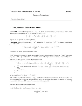
Faster Johnson-Lindenstrauss style reductions Introduction The Johnson-Lindenstrauss Lemma The Johnson-Lindenstrauss Lemma The Johnson-Lindenstrauss Lemma [5] is the archetypal result for ℓ 2 dimensionality reduction Tells us that for n points, there is an ǫ -embedding of 2 → ℓ O (log n /ǫ 2 ) ℓ d 2 Theorem Suppose { u i } i =1 ... n ∈ R n × d . Then, for ǫ > 0 and k = O (log n /ǫ 2 ) , there is a mapping f : R d → R k so that ( ∀ i , j )(1 − ǫ ) || u i − u j || 2 ≤ || f ( u i ) − f ( u j ) || 2 ≤ (1 + ǫ ) || u i − u j || 2

Faster Johnson-Lindenstrauss style reductions Introduction The Johnson-Lindenstrauss Lemma Johnson-Lindenstrauss in practice Proof of Johnson-Lindenstrauss lemma is non-constructive (unfortunately!) In practise, we use the probabilistic method to do a Johnson-Lindenstrauss style reduction Insert randomness at the cost of an exact guarantee Now the guarantee becomes probabilistic

Faster Johnson-Lindenstrauss style reductions Introduction The Johnson-Lindenstrauss Lemma Johnson-Lindenstrauss in practice Standard version: Theorem Suppose { u i } i =1 ... n ∈ R n × d . Then, for ǫ > 0 and 1 k = O ( β log n /ǫ 2 ) , the mapping f ( u i ) = k u i R, where R is a √ d × k matrix of i.i.d. Gaussian variables, satisfies with probability at least 1 − 1 n β , ( ∀ i , j )(1 − ǫ ) || u i − u j || 2 ≤ || f ( u i ) − f ( u j ) || 2 ≤ (1 + ǫ ) || u i − u j || 2

Faster Johnson-Lindenstrauss style reductions Introduction Speeding up computation Achlioptas’ improvement Achlioptas [1] gave an ever simpler matrix construction:  probability = 1  +1  √ 6 probability = 2 R ij = 3 0 3   probability = 1 − 1 6 2 3 rds sparse, and simpler to construct than a Gaussian matrix With no loss in accuracy!

Faster Johnson-Lindenstrauss style reductions Introduction Speeding up computation A question 2 3 rds sparsity is a good speedup in practise But density is still O ( dk ) Computing the mapping is still an O ( dk ) operation asymptotically Let A = { A : ∀ unit x ∈ R d , with v.h.p., (1 − ǫ ) ≤ || A x || 2 ≤ (1+ ǫ ) } Question : For which A ∈ A can A x be computed quicker than O ( dk )?

Faster Johnson-Lindenstrauss style reductions Introduction Speeding up computation The answer? We look at two approaches that allow for quicker computation First is the Fast Johnson-Lindenstrauss transform , based on a Fourier transform Next is the Ailon-Liberty Transform , based on a Fourier transform and error correcting codes!

Faster Johnson-Lindenstrauss style reductions The Fast Johnson-Lindenstrauss Transform The Fast Johnson-Lindenstrauss Transform Ailon and Chazelle [2] proposed the Fast Johnson-Lindenstrauss transform Can speedup ℓ 2 reduction from O ( dk ) to (roughly) O ( d log d ) How? Make the projection matrix even sparser Need some “tricks” to solve the problems associated with this Let’s reverse engineer the construction...

Faster Johnson-Lindenstrauss style reductions The Fast Johnson-Lindenstrauss Transform Sparser projections Sparser projection matrix Use the projection matrix � � � 0 , 1 N p = q q P ∼ 0 p = 1 − q where � � log 2 n � � q = min Θ , 1 d � 1 � �� log 3 n , d log n Density of the matrix is O ǫ 2 min In practise, this is typically significantly sparser than Achlioptas’ matrix

Faster Johnson-Lindenstrauss style reductions The Fast Johnson-Lindenstrauss Transform Trouble with sparse vectors? What do we lose? Can follow standard concentration-proof methods But we end up needing to assume that || x || ∞ is bounded - namely, that information is spread out We fail on vectors like x = (1 , 0 , . . . , 0) i.e. sparse data and a sparse projection don’t mix well So are we forced to choose between generality or usefulness?

Faster Johnson-Lindenstrauss style reductions The Fast Johnson-Lindenstrauss Transform Trouble with sparse vectors? What do we lose? Can follow standard concentration-proof methods But we end up needing to assume that || x || ∞ is bounded - namely, that information is spread out We fail on vectors like x = (1 , 0 , . . . , 0) i.e. sparse data and a sparse projection don’t mix well So are we forced to choose between generality or usefulness? Not if we try to insert randomness...

Faster Johnson-Lindenstrauss style reductions The Fast Johnson-Lindenstrauss Transform Trouble with sparse vectors? A clever idea Can we randomly transform x so that || Φ( x ) || 2 = || x || 2 || Φ( x ) || ∞ is bounded with v.h.p.?

Faster Johnson-Lindenstrauss style reductions The Fast Johnson-Lindenstrauss Transform Trouble with sparse vectors? A clever idea Can we randomly transform x so that || Φ( x ) || 2 = || x || 2 || Φ( x ) || ∞ is bounded with v.h.p.? Answer : Yes! Use a Fourier transform Φ = F Distance preserving Has an “uncertainty principle” - a “signal” and its Fourier transform cannot both be concentrated Use the FFT to give an O ( d log d ) random mapping Details on the specifics in next section...

Faster Johnson-Lindenstrauss style reductions The Fast Johnson-Lindenstrauss Transform Trouble with sparse vectors? Applying a Fourier transform Fourier transform will guarantee that || x || ∞ = ω (1) ⇐ ⇒ || � x || ∞ = o (1) But now we will be in trouble if the input is uniformly distributed! To deal with this, do a random sign change: � x = D x where D is a random diagonal ± 1 matrix Now we get a guarantee of spread with high probability, so the “random” Fourier transform gives us back generality

Faster Johnson-Lindenstrauss style reductions The Fast Johnson-Lindenstrauss Transform Trouble with sparse vectors? Random sign change The sign change mapping D x will give us     d 1 x 1 ± x 1     d 2 x 2 ± x 2     � x =  =  .   .  . .    . . d d x d ± x d where the ± are attained with equal probability Clearly norm preserving

Faster Johnson-Lindenstrauss style reductions The Fast Johnson-Lindenstrauss Transform Trouble with sparse vectors? Putting it together So, we compute the mapping f : x �→ P F ( D x ) Runtime will be � � d log n �� , log 3 n O d log d + min ǫ 2 ǫ 2 Under some loose conditions, runtime is � � d log d , k 3 �� O max � � √ If k ∈ Ω(log d ) , O ( d ) , this is quicker than the O ( dk ) simple mapping In practise, upper bound is reasonable, lower bound might not be though

Faster Johnson-Lindenstrauss style reductions The Fast Johnson-Lindenstrauss Transform Summary Summary Tried increasing sparsity with disregard for generality Used randomization to get back generality (probabilistically) Key ingredient was a Fourier transform, with a randomization step first

Faster Johnson-Lindenstrauss style reductions Ailon and Liberty’s improvement Ailon and Liberty’s improvement Ailon and Liberty [3] improved the runtime from O ( d log d ) to � d 1 / 2 − δ � O ( d log k ), for k = O , δ > 0 Idea : Sparsity isn’t the only way to speedup computation time Can also speedup runtime when the projection matrix has a special structure So find a matrix with a convenient structure and which will satisfy the JL property

Faster Johnson-Lindenstrauss style reductions Ailon and Liberty’s improvement Operator norm We need something called the operator norm in our analysis The operator norm of a transformation matrix A is || A || p → q = sup || A x || q || x || p =1 i.e. maximal q norm of the transformation of unit ℓ p -norm points A fact we will need to employ: || A || p 1 → p 2 = || A T || q 2 → q 1 p 1 + 1 1 q 1 = 1 , 1 p 2 + 1 where q 2 = 1