Sparse Approximate Inverse and Hybrid Algorithms for Matrix - PowerPoint PPT Presentation
www.bsc.es On Scalability Behaviour of Monte Carlo Sparse Approximate Inverse and Hybrid Algorithms for Matrix Computations Vassil Alexandrov (ICREA-BSC) SOFIA 2013, Overview About BSC HPC trends Monte Carlo History and Motivation
www.bsc.es On Scalability Behaviour of Monte Carlo Sparse Approximate Inverse and Hybrid Algorithms for Matrix Computations Vassil Alexandrov (ICREA-BSC) SOFIA 2013,
Overview About BSC HPC trends Monte Carlo – History and Motivation Parallel Algorithm Scaling behaviour Monte Carlo , SPAI and MSPAI Experimental results Conclusions 2
BSC OVERVIEW
Barcelona Supercomputing Center The BSC-CNS (over 350 researchers) objectives: R&D in Computer Sciences, Life Sciences and Earth Sciences Supercomputing support to external research Extreme Computing Application scope Solving Problems “Life Sciences” With Uncertainty, Exascale Computing Application scope Compilers and “Earth Sciences” tuning of application kernels Programming models and Application scope performance “Astrophysics” tuning tools Architectures and hardware Application scope technologies “Engineering” Application scope “Physics”
BSC Four joint centres/institutes: IBM, Intel, Microsoft, CUDA Severo Ochoa excellence award from Spanish Government PRACE - PATC training centre 62 European and national grants 5
MareNostrum III IBM iDataPlex cluster with 3028 compute nodes • Peak Performance of 1 Petaflops • 48,448 Intel SandyBridge-EP E5-2670 cores at 2.6 GHz • Two 8 core CPUs per node (16 cores/node) • 94.625 TB of main memory (32 GB/node) • 1.9 PB of disk storage • Interconnection networks: • Infiniband • Gigabit Ethernet • Operating System: Linux - SuSe Distribution • Consisting of 36 racks • Footprint:120m 2 Completed system - 48,448 cores and predicted to be in the top 25 6
MinoTauro NVIDIA GPU cluster with 128 Bull B505 blades • 2 Intel E5649 6-Core processors at 2.53 GHz per node; in total 5544 cores • 2 M2090 NVIDIA GPU Cards • 24 GB of Main memory • Peak Performance: 185.78 TFlops • 250 GB SSD (Solid State Disk) as local storage • 2 Infiniband QDR (40 Gbit each) to a non- blocking network • RedHat Linux • 14 links of 10 GbitEth to connect to BSC GPFS Storage The Green 500 list November 2012: #36 with 1266 Mflops/Watt, 81.5 kW total Power 7
HPC TRENDS
Projected Performance Development
Road to Exascale Prof. Jack Dongarra, ScalA12, SLC, USA
MONTE CARLO METHODS FOR LINEAR ALGEBRA
History – Serial Monte Carlo methods for matrix computation Curtis - 1956 Halton – 1970s Michailov – 1980s Ermakov – 1980s Alexandrov, Fathi 1996-2000 – hybrid methods Sabelfeld – 1990s and 2009 14
History – Parallel Monte Carlo methods for matrix computation Alexandrov, Megson – 1994 O(nNT) Alexandrov, Fathi – 1998-2000 Alexandrov, Dimov – 1998-2002 resolvent MC Alexandrov, Weihrauch, Branford – 2000-2008 Karaivanova – 2000’s - QMC Alexandrov, Dimov, Weichrauch, Branford – 2005-2009 Alexandrov, Strassburg, 2010-2013 – hybrid methods 15
Motivation Many scientific and engineering problems revolve around: – inverting a real n by n matrix (MI) • Given A • Find A -1 – solving a system of linear algebraic equations (SLAE) • Given A and b • Solve for x, Ax = b • Or find A −1 and calculate x = A −1 b 16
Motivation cont . Traditional Methods for dense matrices: – Gaussian elimination – Gauss-Jordan – Both take O(n 3 ) steps Time prohibitive if – large problem size – real-time solution required 17
Idea of the Monte Carlo method Wish to estimate the quantity α Define a random variable ξ Where ξ has the mathematical expectation α Take N independent realisations ξi of ξ – Then – And 18
Reason for using Monte Carlo O(NT) steps to find an element of the – matrix inverse A – solution vector x Where – N Number of Markov Chains – T length of Markov Chains Independent of n - size of matrix or problem Algorithms can be efficiently parallelised 19
MC Important Properties Efficient Distribution of the compute data Minimum communication/ communication reducing algorithms Increased precision is achieved adding extra computations (without restart) Fault-Tolerance achieved through adding extra computations
Parallel Algorithm Start with a diagonally dominant matrix ^B Make the split ^B = D - B 1 – D is the diagonal elements of ^B – B1 has off-diagonal elements only Compute A = D -1 B 1 If we had started with a matrix B that was not diagonally dominant then an additional splitting would have been made at the beginning, B = ^B - (^B - B), and a recovery section would be needed at the end of the algorithm to get B -1 from ^B -1 21
Parallel Algorithm cont. Finding ^B -1 22
Parallel Algorithm cont. Matrix Inversion using MCMC 23
Parallel Algorithm cont. Matrix Setup Use parallel Monte Carlo to find a rough inverse of A Use parallel iterative refinement to improve accuracy and retrieve final inverse 24
Parallel Algorithm cont. 25
Parallel Algorithm cont. Almost linear speedup for large enough problem sizes Minimal inter-process communication necessary Work and communication balanced Smaller problem sizes suffer due to computation/communication ratio 26
HPC SIMULATION
Motivation Predict behaviour on different system Find bottlenecks, sweet spot, scaling problems Easier than running on several machines Reproducible
xSim – The Extreme-Scale Simulator Developed at the Oak Ridge National Laboratory (ORNL), USA Real life application testing and algorithmic resilience options development (Extreme Computing Group at BSC and Computer Science and Mathematics Division at ORNL) Highly scalable solution that trades off accuracy for node oversubscription simulation Execution of real applications, algorithms or their models atop a simulated HPC environment for – Performance evaluation, including identification of resource contention and underutilization issues – Investigation at extreme scale, beyond the capabilities of existing simulation efforts
xSim – The Extreme-Scale Simulator The simulator is a library Virtual processors expose a virtual MPI to applications using a Parallel Discreet Event Simulation (PDES) Easy to use: – Replace the MPI header – Compile and link with the simulator library – Run the MPI program Support for C and Fortran MPI applications
Scaling Behaviour Core Scaling on a 240 core system 31
Scaling Behaviour cont. Core Scaling, logarithmic 32
Scaling Behaviour cont. Problem scaling 33
MONTE CARLO AND SPAI
Combination of Monte Carlo and SPAI SPAI – SParse Approximate Inverse Preconditioner – Computes a sparse approximate inverse M of given matrix A by minimizing ∥ AM − I ∥ in the Frobenius norm – Explicitly computed and can be used as a preconditioner to an iterative method – Uses BICGSTAB algorithm to solve systems of linear algebraic equations Ax = b Sparse Monte Carlo Matrix Inverse Algorithm – Computes an approximate inverse by using Monte Carlo methods – Uses an iterative filter refinement to retrieve the inverse 35
Combination of Monte Carlo and SPAI cont. Idea: using a Monte Carlo computed approximate matrix inverse as a preconditioner – Considering • computation time for MC solution • Suitability of rough inverse • Matrix types that are not invertable via Frobenius norm 36
Experiments Preliminary results – optimisation of parameters necessary Randomly generated sparse and dense matrices Standard SPAI settings – RHS taken from input matrix Monte Carlo method without filter option – Very rough inverse that already provides a good alternative 37
Experiments Computation time in seconds for both preconditioners 8 7 Frobenius 6 Monte Carlo 5 4 8 3 7 2 Frobenius 6 1 Monte Carlo 5 0 50 100 150 200 250 500 1000 2000 3000 4000 5000 4 Sparsity 0.5 3 2 1 0 50 100 150 200 250 500 1000 2000 3000 4000 5000 Sparsity 0.7 38
Experiments cont. Residual from BICGSTAB solution in SPAI 1.00E-02 9.00E-03 8.00E-03 7.00E-03 6.00E-03 5.00E-03 4.00E-03 Frobenius 3.00E-03 Monte Carlo 2.00E-03 1.20E-02 1.00E-03 1.00E-02 0.00E+00 50 100 150 200 250 500 1000 2000 3000 4000 5000 Sparsity 0.5 8.00E-03 6.00E-03 4.00E-03 2.00E-03 0.00E+00 50 100 150 200 250 500 1000 2000 3000 4000 5000 39 Sparsity 0.7
MC & SPAI 40
MC & SPAI residuals 41
Monte Carlo, SPAI & MSPAI 42
43
MONTE CARLO AND MSPAI
Monte Carlo & MSPAI 45
Comparison Monte Carlo - MSPAI University of Florida Sparse Matrix Collection Symmetric Matrix from Parsec set n=268,000 nnz=18,5mio
Residuals for Parsec data set
Runtime for Si10H16
www.bsc.es Thank you! 49
Recommend
More recommend
Explore More Topics
Stay informed with curated content and fresh updates.
