Solutions for Coursework I CS-270, 2011/12 Oliver Kullmann - PDF document

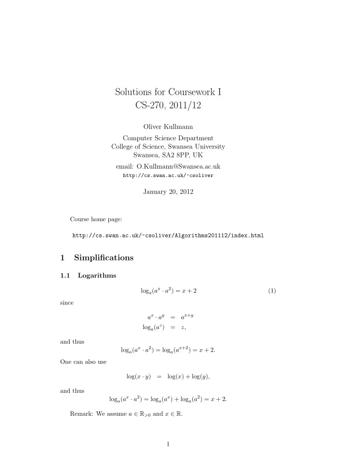
Solutions for Coursework I CS-270, 2011/12 Oliver Kullmann Computer Science Department College of Science, Swansea University Swansea, SA2 8PP, UK email: O.Kullmann@Swansea.ac.uk http://cs.swan.ac.uk/~csoliver January 20, 2012 Course home page: http://cs.swan.ac.uk/~csoliver/Algorithms201112/index.html 1 Simplifications 1.1 Logarithms log a ( a x · a 2 ) = x + 2 (1) since a x · a y a x + y = log a ( a z ) = z, and thus log a ( a x · a 2 ) = log a ( a x +2 ) = x + 2 . One can also use log( x · y ) = log( x ) + log( y ) , and thus log a ( a x · a 2 ) = log a ( a x ) + log a ( a 2 ) = x + 2 . Remark: We assume a ∈ R > 0 and x ∈ R . 1

1.2 Floors and ceilings For n ∈ N 0 we have ⌈ n 2 ⌉ + ⌊ n 2 ⌋ = n. (2) Small examples: ⌈ 0 2 ⌉ + ⌊ 0 2 ⌋ = 0 + 0 = 0 ⌈ 1 2 ⌉ + ⌊ 1 2 ⌋ = 1 + 0 = 1 ⌈ 2 2 ⌉ + ⌊ 2 2 ⌋ = 1 + 1 = 2 ⌈ 3 2 ⌉ + ⌊ 3 2 ⌋ = 2 + 1 = 3 ⌈ 4 2 ⌉ + ⌊ 4 2 ⌋ = 2 + 2 = 4 ⌈ 5 2 ⌉ + ⌊ 5 2 ⌋ = 3 + 2 = 5 . We see: • For even n we have ⌈ n 2 ⌉ = n 2 = ⌊ n 2 ⌋ , since 2 divides n , and thus n 2 is an integer (recall that for integers z we have ⌊ z ⌋ = ⌈ z ⌉ = z ). It follows that for even n we have ⌈ n 2 ⌉ + ⌊ n 2 ⌋ = n 2 + n 2 = n . • For odd n we have ⌈ n 2 ⌉ = n +1 and ⌊ n 2 ⌋ = n − 1 2 , since n − 1 2 , n +1 are integers 2 2 (due to n odd) with n − 1 = n 2 − 1 2 < n 2 < n 2 + 1 2 = n + 1 . 2 2 It follows that for odd n we have ⌈ n 2 ⌉ + ⌊ n 2 ⌋ = n +1 + n − 1 = n . 2 2 1.3 Sums For n ∈ N 0 we have n ( i 2 − ( i − 1) 2 ) = n 2 . � (3) i =1 2

Small examples: 0 ( i 2 − ( i − 1) 2 ) � = 0 i =1 1 ( i 2 − ( i − 1) 2 ) (1 2 − 0 2 ) = 1 � = i =1 2 ( i 2 − ( i − 1) 2 ) (2 2 − 1 2 ) + 1 = 4 � = i =1 3 ( i 2 − ( i − 1) 2 ) (3 2 − 2 2 ) + 4 = 9 � = i =1 4 ( i 2 − ( i − 1) 2 ) (4 2 − 3 2 ) + 9 = 16 . � = i =1 Thus we can guess that the sum evaluates to n 2 . Prove by induction is easy, or one uses directly a telescope sum argument (exploiting cancellation of neigh- bouring terms): n ( i 2 − ( i − 1) 2 ) = � i =1 (( n 2 − ( n − 1) 2 ) + (( n − 1) 2 − ( n − 2) 2 ) + (( n − 2) 2 − ( n − 3) 3 ) + · · · + (1 2 − 0 2 ) = n 2 − 0 2 = n 2 . 2 Theta-Expressions 5 n 3 − 6 n 2 + | sin( n ) | = Θ( n 3 ) � (4) since terms of lower order can be removed, and we have 5 n 3 Θ( n 3 ) = 6 n 2 Θ( n 2 ) = � | sin( n ) | = Θ(1) . 2 n + n 1000 = Θ(2 n ) (5) since for every a and every b > 1 we have n a = O ( b n ) (exponential growth is asymptotically stronger than polynomial growth), and thus one can argue 2 n + n 1000 = 2 n + O (2 n ) = O (2 n ) 2 n + n 1000 = Ω(2 n ) . 3

2 n + 3 n = Θ(3 n ) (6) since for n ≥ 0 we have 2 n ≤ 3 n , and thus 2 n + 3 n ≤ 2 · 3 n = O (3 n ) 2 n + 3 n = Ω(3 n ) . 3 Growth order We have • 2 lg n = n • √ n = n 1 2 log2 n 1 1 log 2 10 , and thus 2 log 10 n = 2 log 2 n log2 10 = (2 log 2 n ) log2 10 = n log2 10 , • log 10 n = where log 2 10 > 3 since 2 3 = 8 < 10. • 2 n > n for n ≥ 0, and thus 2 ( n 2 ) = (2 n ) n > n n . So the sorting of the given functions (of n ) by ascending order of growth is 2 log 10 n , √ n, 2 lg n , n 2 , n 3 , 2 n , e n , n ! , n n , 2 ( n 2 ) . Remarks: • We use lg( x ) = log 2 ( x ) (common is also ld( x ) = log 2 ( x ) for “logarithm dualis”). • Common is ln( x ) = log e ( x ) with e = 2 . 71828182845904 . . . (for “logarithm naturalis”). • When we use log( x ), then typically the basis of the logarithm is left “open”. For example in log a ( x ) = log( x ) log( a ) , where on the right-hand side actually any basis can be used (but consis- tently!), that is, more precisely we have for every a, b > 1: log a ( x ) = log b ( x ) log b ( a ) . 4

4 Master theorem T ( n ) = 3 T ( n ⇒ T ( n ) = Θ( n log 2 3 ) . 2 ) + 5 = (7) This is case 1 of the Master Theorem, with a = 3, b = 2 and c = 0. We can also write it as T ( n ) = 2 log 2 3 T ( n 2 ) + Θ(1). T ( n ) = 16 T ( n 4 ) + n 2 = ⇒ T ( n ) = Θ( n 2 · log n ) . (8) This is case 2, with a = 16, b = 4 and c = 2. We can also write it as T ( n ) = 4 2 T ( n 4 ) + n 2 . 2 ) + √ n = ⇒ T ( n ) = Θ( √ n ) . T ( n ) = T ( n (9) This is case 3, with a = 1, b = 2 and c = 1 2 . We can also write it as T ( n ) = 1 2 0 T ( n 2 . 2 ) + n 5 Sorting 4 numbers When using insertion-sort for sorting 3 numbers, we need 2+1 = 3 comparisons. In general, for n items, we need (precisely) n − 1 i = 1 � 2 n ( n − 1) i =1 comparisons. This can be achieved also by the following simple function (using C with reference-parameters): void sort3 ( int & a , int & b , int & c ) { i f (b < a ) swap (a , b ) ; i f ( c < b) swap (b , c ) ; i f (b < a ) swap (a , b ) ; } The key ideas for sorting 4 numbers a, b, c, d with (only) 5 comparisons are: 1. Sort the first three numbers a, b, c with 3 comparisons. 2. Compare d with the middle number b : then only further comparison with a resp. c is needed. The C++-code is as follows (this time not modifying the arguments, but re- turning a vector with 4 elements): 5

vector < int > sort4 ( int a , int b , int c , const int d) { sort3 (a , b , c ) ; // now a < = b < = c i f (d < b) { i f (d < a ) return { d , a , b , c } ; return { a , d , b , c } ; } i f (d < c ) return { a , b , d , c } ; return { a , b , c , d } ; } 6 Analysing Insertion-Sort The number of inversions of an array A of length n ≥ 1, denoted here by inv( A ) , is the number of pairs ( i, j ) with 1 ≤ i < j ≤ n and A [ i ] > A [ j ]. (In the solution we drop the simplifying assumptions that A is repetition-free.) The inversions of (2 , 3 , 8 , 6 , 1) are (1 , 5) , (2 , 5) , (3 , 4) , (3 , 5) , (4 , 5) . When there are no duplicate elements in A, then for readability we can write the elements instead of the indices: (2 , 1) , (3 , 1) , (8 , 6) , (8 , 1) , (6 , 1) . Amongst the arrays with n elements, the array ( n, n − 1 , . . . , 1) has the maximal number of inversions, namely n − 1 i = 1 � ( n − 1) + ( n − 2) + · · · + 1 + 0 = 2 n ( n − 1) . i =1 This is maximal over all arrays (which might contain repetitions), which can be proven by induction: • The statement is true for n = 1 (zero inversions). • Assume n > 1, and that it is true for length n − 1. Consider any array A = ( a 1 , . . . , a n ). Without loss of generality we can assume { a 1 , . . . , a n } = { 1 , . . . , n } . (Essential here the claim (in the “without loss of generality”) that repe- titions of values do not increase the number of inversions. That actually needs a proof. Harmless is the renaming, bringing arbitrary values into the range from 1 to n .) • Now the number of inversions of A is not decreased if we bring n to the front. So without loss of generality we can assume a 1 = n . 6

• Now we can apply the induction hypothesis to ( a 2 , . . . , a n ) and deduce that there can be at most 1 2 ( n − 1)( n − 2) inversions in it. • a 1 contributes further n − 1 inversions, and so altogether we have at most 1 2 ( n − 1)( n − 2) + ( n − 1) = ( n − 1)( 1 2 ( n − 2) + 1) = ( n − 1) 1 2 n inversions. QED Recall the analysis of insertion-sort in week 1: 1. Eight different operations were identified, with associated costs c 1 , . . . , c 8 , corresponding to the eight lines of code. (These c i are parameters, depend- ing on the execution environment; only c 3 is known in advance, namely c 3 = 0.) 2. The total run-time on input A is (precisely) n n � � T ( A ) = c 1 · n +( c 2 + c 4 + c 8 ) · ( n − 1)+ c 5 · t j +( c 6 + c 7 ) · ( t j − 1) = j =2 j =2 n � c 1 · n + ( c 2 + c 4 + c 8 − c 6 − c 7 ) · ( n − 1) + ( c 5 + c 6 + c 7 ) · t j . j =2 3. The number t j for j ∈ { 2 , . . . , n } here is just the number of executions of line 5 (the while -check) for the execution of the outer loop with loop- variable value j . The crucial observation now is that t j is 1 plus the number of inversions A [ j ] is involved which are to the left of position j . We get n � t j = inv( A ) + n − 1 . j =2 So T ( A ) = c 1 · n +( c 2 + c 4 + c 8 − c 6 − c 7 ) · ( n − 1)+( c 5 + c 6 + c 7 ) · (inv( A )+ n − 1) = c 1 · n + ( c 2 + c 4 + c 5 + c 8 ) · ( n − 1) + ( c 5 + c 6 + c 7 ) · inv( A ) = ( c 5 + c 6 + c 7 ) · inv( A ) + ( c 1 + c 2 + c 4 + c 5 + c 8 ) · n − ( c 2 + c 4 + c 5 + c 8 ) . Thus the run-time of insertion sort on input A is Θ( n + inv( A )) . (Note that this means here that there a constants α, β , depending on the execution envi- ronment, such that α · ( n + inv( A )) ≤ T ( A ) ≤ β · ( n + inv( A )). Also note that here we have the precise dependency on the input, not just on the input-length n , and so it’s not a worst-case statement, but an exact-case statement.) Finally let’s consider how to computer inv( A ). We could compute it via insertion-sort in time O ( n 2 ). Can we do better? 7