Definition Recursion See "Recursion". Recursion If you - PDF document

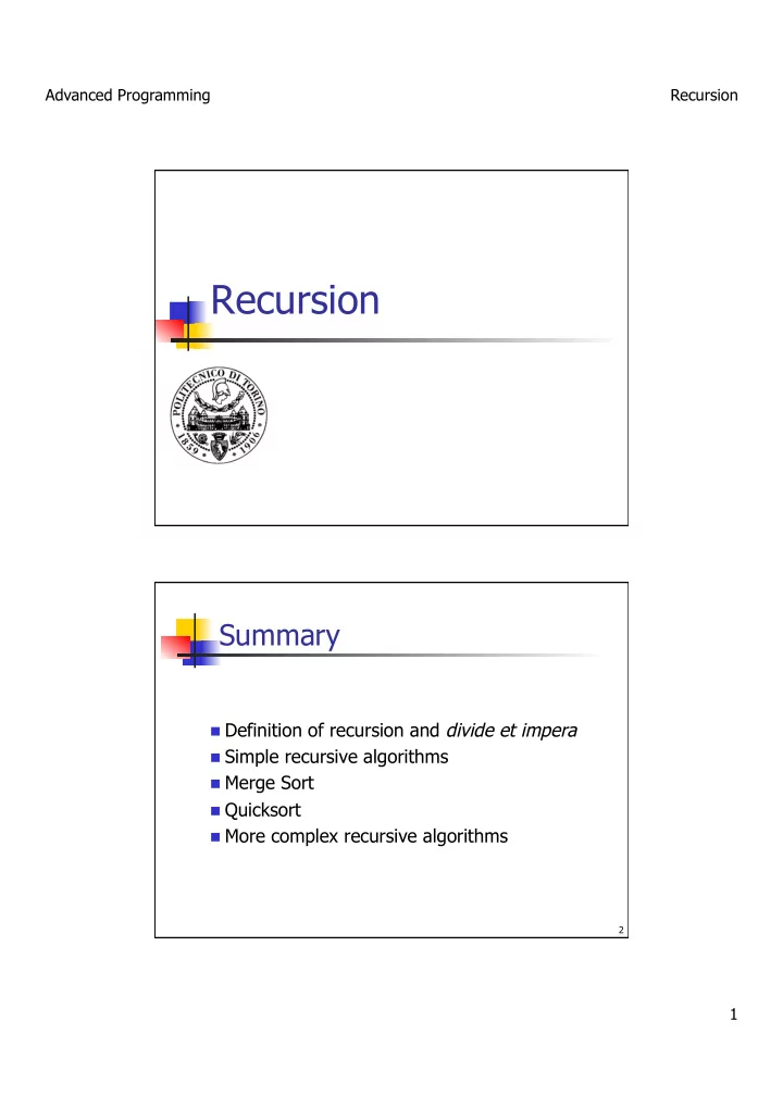
Advanced Programming Recursion Recursion Summary n Definition of recursion and divide et impera n Simple recursive algorithms n Merge Sort n Quicksort n More complex recursive algorithms 2 1

Advanced Programming Recursion Definition Recursion See "Recursion". Recursion If you still don't get it, see: "Recursion". J 3 Definition n A function F is called recursive when: 1 Within the F function definition, there is a call to the same F function 2 or there is a call to a function G which calls, directly or indirectly, the function F. n An algorithm is called recursive when it is based on recursive functions. 4 2

Advanced Programming Recursion Examples 5 Example: factorial double fact( double N ) n 0! ≡ 1 { if(N == 0) n ∀ N ≥ 1 : return 1.0 ; N! ≡ N ⋅ (N-1)! return N * fact( N-1 ); } 6 3

Advanced Programming Recursion Motivation n Many problems have a recursive nature: n Define a method for solving sub-problems similar to the initial one (but smaller) n Define a method to combine partial solutions in the whole solution of the initial problem. 7 “ a ” sub-problems, Divide and Conquer each one “ b ” times smaller than the problem n Solution = Solve (problem) ; n Solve (problem): n Subproblem 1,2,3,…,a = Divide(problem) ; n For each subproblem i : n Sub-solution i = Solve(subproblem i ) ; n Return solution = Combine(sub-solution 1,2,3,…,a ) ; 8 4

Advanced Programming Recursion Divide and Conquer Recursive call n Solution = Solve(problem) ; n Solve (problem): n Subproblem 1,2,3,…,a = Divide(problem) ; n For each subproblem i : n Sub-solution i = Solve (subproblem i ) ; n Return solution = Combine(sub-solution 1,2,3,…,a ) ; 9 When stopping? Recursion must not be infinite, as an algorithm must stop eventually… At some point, sub-problems become so simple to be solvable because: n Obvious solution, in case of sets of only one element n Methods alternative to recursion. 10 5

Advanced Programming Recursion Note Well n Remember to always set a stop condition n Try to make sub-problems dimensions less than the initial problem 11 Divide and Conquer (with stop condition) Solve(problem): n If the problem is simple: n Solution = Solve_simple( problem ) n Else: n Sub-problem 1,2,3,…,a = Divide(problem) ; n Fro each sub-problem i : n Sub-solution i = Solve(subproblem i ) ; n Return solution = Combine (subsolution 1,2,3,…,a ); 12 6

Advanced Programming Recursion Complexity (I) T(n) Solve (problem): Θ (1) n If the problem is simple (n ≤ c): n Solution = Solve_simple(problem) D(n) n Else: n Sub-problem 1,2,3,…,a = Divide(problem) ; n For each subproblem i : T(n/b) n Subsolution i = Solve(subproblem i ) ; n Return solution = Combine(subsolution 1,2,3,…,a ) ; C(n) 13 Complexity (II) T(n) = n Θ (1) for n ≤ c n D(n) + a T(n/b) + C(n) for n > c Recursive Equation not easy to solve. If D(n)+C(n)= Θ (n), then T(n)= Θ (n log n). 14 7

Advanced Programming Recursion Summary n Definition of recursion and divide et impera n Simple recursive algorithms n Merge Sort n Quicksort n More complex recursive algorithms 15 Example: Fibonacci numbers Problem: n Calculate the N-th number of Fibonacci sequence Definition: n FIB N+1 = FIB N + FIB N-1 for n>0 n FIB 1 = 1 n FIB 0 = 0 16 8

Advanced Programming Recursion Solution long fib(int N) { long f1, f2 ; if(N == 0) return 0 ; if(N == 1) return 1 ; f1 = fib(N-1) ; f2 = fib(N-2) ; return f1+f2 ; } 17 Analysis FIB(5) FIB(3) FIB(4) FIB(1) FIB(2) FIB(3) FIB(2) FIB(0) FIB(1) FIB(1) FIB(2) FIB(1) FIB(0) FIB(1) FIB(0) 18 9

Advanced Programming Recursion Example: binary search Problem n Define if an element x is included in a sorted array v[N] Approach n Divide the array in 2 half parts and re-apply the problem on one half (the other half can be excluded as the array is sorted) 19 Example v x 1 3 4 6 8 9 11 12 4 1 3 4 6 8 9 11 12 1 3 4 6 y y ≥ x y<x 4 6 20 10

Advanced Programming Recursion Solution int search(int v[], int a, int b, int x) { int c ; if(b-a == 0) if (v[a]==x) return a ; else return –1 ; c = (a+b) / 2 ; if(v[c] >= x) return search(v, a, c, x) ; else return search(v, c+1, b, x) ; } 21 Binary search v 1 3 4 6 8 9 11 12 6 2 h ≤ n < 2 h+1 3 9 h h = ⎣ log 2 (n) ⎦ 1 4 8 11 12 22 11

Advanced Programming Recursion Binary search v 1 3 4 6 8 9 11 12 6 2 h ≤ n < 2 h+1 3 9 h h = ⎣ log 2 (n) ⎦ 1 4 8 11 At most h nodes of the (virtual) tree 12 are visited to find the searched element 23 Exercise Calculate binomial coefficient (n m), taking into account information derived from Tartaglia triangle: n n 1 n 1 ⎧ − ⎛ − ⎛ ⎞ ⎛ ⎞ ⎞ ⎜ ⎟ ⎜ ⎟ ⎜ ⎟ = + ⎪ ⎜ ⎟ ⎜ ⎟ ⎜ ⎟ m m 1 m − ⎝ ⎠ ⎝ ⎠ ⎝ ⎠ ⎪ ⎪ n n ⎛ ⎞ ⎛ ⎞ ⎨ 1 ⎜ ⎟ = ⎜ ⎟ = ⎜ ⎟ ⎜ ⎟ ⎪ n 0 ⎝ ⎠ ⎝ ⎠ ⎪ 0 n , 0 m n ⎪ ≤ ≤ ≤ ⎩ 24 12

Advanced Programming Recursion Exercise Calculate the determinant of a square matrix. Remember that: n Det(M 1x1 ) = m 11 n Det(M NxN ) = sum of products of elements of a row (or column) multiplied the determinants of sub-matrixes (N-1)x(N-1) obtained by deleting the row and column containing the element, taken with sign (-1) i+j . 25 Recursion and iteration An Information Theory theorem proves that each recursive program can be implemented with an iterative program. Best solution may depend on efficiency and clarity of code and it depends by the kind of problem. 26 13

Advanced Programming Recursion Example: factorial (iterative) double fact( double N ) { n 0! ≡ 1 double tot = 1.0 ; int i; n ∀ N ≥ 1 : for(i=2; i<=N; ++i) N! ≡ N ⋅ (N-1)! tot = tot * i ; return tot ; } 27 Fibonacci (iterative) long fib(int N) { long f1=1, f2=0, f ; int i; if(N == 0) return 0 ; if(N == 1) return 1 ; f = f1 + f2 ; /* N==2 */ for(i=3; i<= N; ++i) { f2 = f1 ; f1 = f ; f = f1+f2 ; } return f ; } 28 14

Advanced Programming Recursion Binary Search (iterative) int search(int v[], int a, int b, int x) { int c ; while(b-a != 0) { c = (a+b) / 2 ; if(v[c] >= x) b = c ; else a = c+1 ; } if(v[a]==x) return a ; else return –1 ; } 29 Proposed Excercises 1. Provide the iterative version of binomial coefficient (n m). 2. Analyze the difficulties in realizing the iterative version of determinant calculation. 30 15

Advanced Programming Recursion Sorting Algorithms (Recursive Algorithms) Summary n Definition of recursion and divide et impera n Simple recursive algorithms n Merge Sort n Quicksort n More complex recursive algorithms 32 16

Advanced Programming Recursion Merge Sort Merge Sort algorithm is the direct application of “ Divide and Conquer ” to sorting problems. 6 12 4 5 2 9 5 12 Divide 6 12 4 5 2 9 5 12 Solve Solve 4 5 6 12 2 5 9 12 Combine 2 4 5 5 6 9 12 12 33 Merge Sort: Divide “ Divide ” step simply consists in partitioning the initial array in 2 sub-arrays, before and after the division point, which is usually chosen in the middle of the array. 1 8 p r 6 12 4 5 2 9 5 12 Divide 6 12 4 5 2 9 5 12 1 4 5 8 p q q+1 r 34 17

Advanced Programming Recursion Merge Sort: stop condition Stop condition holds whenever the sub-array has only one element (p==r) or no elements (p>r). 35 Merge Sort: Combine Combine step is based on merge of two ordered vectors: n Given 2 ordered arrays, merge them together in a third sorted array This algorithm complexity is Θ (n). 4 5 6 12 2 5 9 12 Combine 2 4 5 5 6 9 12 12 36 18

Advanced Programming Recursion Pseudo-code M ERGE- S ORT ( A , p , r ) 1 if p < r Stop condition 2 then q ← ⎣ ( p + r )/2 ⎦ Divide 3 M ERGE- S ORT ( A , p , q ) Solve 4 M ERGE- S ORT ( A , q +1, r ) Combine 5 M ERGE ( A , p , q , r ) 37 Notation These symbols are used in math and computer science: n ⎣ x ⎦ = the biggest integer <= x (read: “floor of x”) n i.e. integer part of x n ⎡ x ⎤ = the smallest integer >= x (read: “ceiling of x”) Examples: n ⎣ 3 ⎦ = ⎡ 3 ⎤ = 3 n ⎣ 3,1 ⎦ = 3; ⎡ 3,1 ⎤ = 4 38 19