Single Period Models (continued) One-step Binary Model Pricing a - PowerPoint PPT Presentation
Single Period Models (continued) One-step Binary Model Pricing a European call maturing at time T on an asset with price S t . Deal is entered at t = 0 at a strike of K , when the asset price is S 0 . Assume S T can take one of only 2
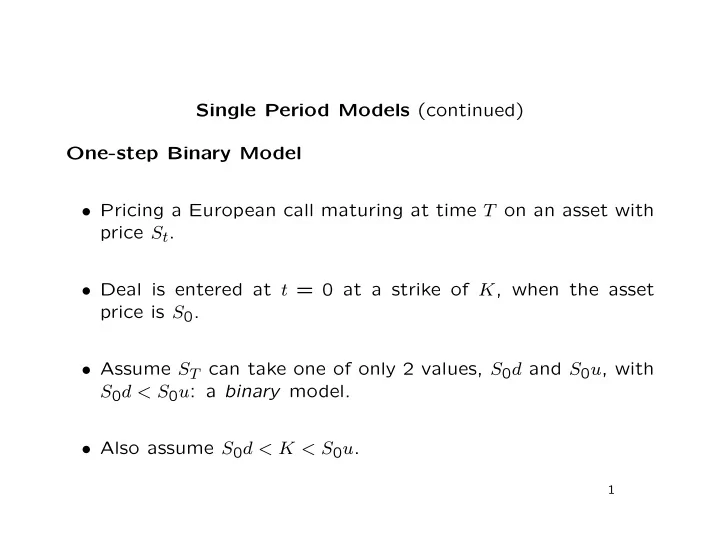
Single Period Models (continued) One-step Binary Model • Pricing a European call maturing at time T on an asset with price S t . • Deal is entered at t = 0 at a strike of K , when the asset price is S 0 . • Assume S T can take one of only 2 values, S 0 d and S 0 u , with S 0 d < S 0 u : a binary model. • Also assume S 0 d < K < S 0 u . 1
• How to replicate? • Try a portfolio of x 1 in cash and x 2 units of the asset, with value at time t V t = x 1 e rt + x 2 S t . • Choose x 1 and x 2 to match the payoff of the call: if S T = S 0 d < K , the payoff is 0, so V T = x 1 e rT + x 2 S 0 d = 0 , and if S T = S 0 u > K , the payoff is S 0 u − K , so V T = x 1 e rT + x 2 S 0 u = S 0 u − K. 2
• Solving: x 1 = − de − rT ( S 0 u − K ) , u − d x 2 = S 0 u − K S 0 ( u − d ) . • We can set up this portfolio at t = 0 with a cost of � 1 − de − rT � ( S 0 u − K ) x 1 + x 2 S 0 = . u − d • If the price of the option is different, an arbitrage is possible, so this is the no-arbitrage price. • Note: no probabilities were needed for the two values of S T . 3
A Ternary Model • We can make the model marginally more realistic by allowing three (or more) values for S T . • For a general European contingent claim with payoff C ( S T ), we now have 3 (or more) equations in the two unkowns x 1 and x 2 , and in general no solution. • That is, some contingent claims cannot be replicated; the market is said to be not complete , and no unique no-arbitrage price exists. 4
Characterization of No Arbitrage • General single-period model, with N assets. • Asset prices at t = 0 are � t ∈ R N . � S 1 0 , S 2 0 , . . . , S N S 0 = 0 • Market has n possible states at t = T . • Price of asset i if, at t = T , market is in state j is D i,j . • That is, prices in state j are the vector D j , column j of the � � N × n matrix D = . D i,j 5
• A portfolio is an investment in these assets with weight θ i on asset i , i = 1 , 2 , . . . , N ; it is defined by θ = ( θ 1 , θ 2 , . . . , θ N ) t ∈ R N . • The value of the portfolio at t = 0 is the scalar product S 1 0 θ 1 + S 2 0 θ 2 + · · · + S N 0 θ N = S 0 · θ . • Similarly the value at t = T , if the market is in state j , is the scalar product D 1 ,j θ 1 + D 2 ,j θ 2 + · · · + D N,j θ N • We can write these as a vector D t θ ∈ R n . 6
Notation: • R n + = { x ∈ R n ; x i ≥ 0 , i = 1 , 2 , . . . , n } ; • for x ∈ R n + , we write x ≥ 0 ; • if x ≥ 0 and x � = 0 , we write x > 0 ; • R n ++ = { x ∈ R n ; x i > 0 , i = 1 , 2 , . . . , n } ; • for x ∈ R n ++ , we write x ≫ 0 . 7
• An arbitrage is a portfolio θ ∈ R N satisfying either S 0 · θ ≤ 0 and D t θ > 0 or S 0 · θ < 0 and D t θ ≥ 0 . • That is, either: – the portfolio costs nothing to set up, loses money in no market state at time T , and gains money in at least one state; or – the portfolio yields cash when it is set up and loses money in no market state. 8
• Characterization: there is no arbitrage if and only if there is a state price vector : a vector ψ ∈ R n ++ such that S 0 = D 1 ψ 1 + D 2 ψ 2 + · · · + D n ψ n = D ψ . • That is, the vector of asset prices at t = 0 is a positively weighted linear combination of the vectors of prices in the various states of the market at t = T . • Proof involves a separating hyperplane theorem and the Riesz representation theorem ; it is basically finite-dimensional con- vex geometry. • Note that the state price vector may not be unique. 9
Recommend
More recommend
Explore More Topics
Stay informed with curated content and fresh updates.
