Single-parameter models: Poisson data Applied Bayesian Statistics - PowerPoint PPT Presentation
Single-parameter models: Poisson data Applied Bayesian Statistics Dr. Earvin Balderama Department of Mathematics & Statistics Loyola University Chicago September 14, 2017 Poisson-Gamma model 1 Last edited September 8, 2017 by Earvin
Single-parameter models: Poisson data Applied Bayesian Statistics Dr. Earvin Balderama Department of Mathematics & Statistics Loyola University Chicago September 14, 2017 Poisson-Gamma model 1 Last edited September 8, 2017 by Earvin Balderama <ebalderama@luc.edu>
One-parameter models The Poisson model Estimating a rate has many applications: Number of new Zika cases per day. Number of invasive trees per square mile. Number of concussions per NFL season. What we observe (the data) is some number of events, Y ∈ { 0 , 1 , 2 , . . . } , that occur over some given time period or spatial region. Let λ > 0 be the rate parameter we are trying to estimate. We would like to obtain the posterior of λ . Poisson-Gamma model 2 Last edited September 8, 2017 by Earvin Balderama <ebalderama@luc.edu>
One-parameter models Bayesian analysis - Likelihood Given a rate λ , the distribution of Y can be described as Y | λ ∼ Poisson ( λ ) Thus, the likelihood function for Y = y is f ( y | λ ) = λ y e − λ y ! Poisson-Gamma model 3 Last edited September 8, 2017 by Earvin Balderama <ebalderama@luc.edu>
One-parameter models Bayesian analysis - Likelihood Given a rate λ , the distribution of Y can be described as Y | λ ∼ Poisson ( λ ) Thus, the likelihood function for Y = y is f ( y | λ ) = λ y e − λ y ! Note: If we consider the observation period or region to be composed of M temporal or spatial units, and λ is the rate per unit, then a more general specification of the likelihood would be Y | λ ∼ Poisson ( M λ ) , and f ( y | λ ) = ( M λ ) y e − M λ y ! Poisson-Gamma model 3 Last edited September 8, 2017 by Earvin Balderama <ebalderama@luc.edu>
One-parameter models Bayesian analysis - Prior λ is the parameter of interest, and is continuous and positive. A natural prior distribution to select would be λ ∼ Gamma ( a , b ) Thus, b a Γ( a ) λ a − 1 e − b λ f ( λ ) = Poisson-Gamma model 4 Last edited September 8, 2017 by Earvin Balderama <ebalderama@luc.edu>
One-parameter models Bayesian analysis - Posterior We can now derive the posterior distribution, which happens to be: λ | Y ∼ Gamma ( a + Y , b + M ) Poisson-Gamma model 5 Last edited September 8, 2017 by Earvin Balderama <ebalderama@luc.edu>
One-parameter models Bayesian analysis - Posterior We can now derive the posterior distribution, which happens to be: λ | Y ∼ Gamma ( a + Y , b + M ) Note: a and b can be interpreted as the “prior number of events and observation time/spatial units,” which may be useful for specifying the prior. What values of a and b to select if we have no information about λ before collecting data? What if historical data/expert opinion indicates that λ is likely between 2 and 4 per day, and data is observed weekly? Poisson-Gamma model 5 Last edited September 8, 2017 by Earvin Balderama <ebalderama@luc.edu>
One-parameter models Likelihood for two observations Suppose our data consists of two independent observations, Y 1 | λ ∼ Poisson ( M λ ) and Y 2 | λ ∼ Poisson ( M λ ) Thus, the likelihood function for Y 1 = y 1 , Y 2 = y 2 is f ( y 1 , y 2 | λ ) = ( M λ ) y 1 e − M λ · ( M λ ) y 2 e − M λ y 1 ! y 2 ! = ( M λ ) y 1 + y 2 e − 2 M λ y 1 ! y 2 ! With a Gamma ( a , b ) prior, the posterior distribution becomes: λ | Y 1 , Y 2 ∼ Gamma ( a + Y 1 + Y 2 , b + 2 M ) Poisson-Gamma model 6 Last edited September 8, 2017 by Earvin Balderama <ebalderama@luc.edu>
One-parameter models Likelihood for n observations Suppose our data consists of n observations, iid Y 1 , . . . , Y n | λ ∼ Poisson ( M λ ) Thus, the likelihood function is n ( M λ ) y i e − M λ � f ( y 1 , . . . , y n | λ ) = y i ! i = 1 � i y i e − nM λ = ( M λ ) � i y i ! With a Gamma ( a , b ) prior, the posterior distribution becomes: � n � � λ | Y 1 , . . . Y n ∼ Gamma a + Y i , b + nM i = 1 Poisson-Gamma model 7 Last edited September 8, 2017 by Earvin Balderama <ebalderama@luc.edu>
One-parameter models Shrinkage The prior mean was E ( λ ) = a b . The posterior mean is λ B = E ( λ | Y 1 , . . . Y n ) = a + � Y i ˆ b + nM �� Y i � b � a � nM = b + b + nM b + nM nM � Y i The posterior mean is between the sample rate nM and the prior mean a b . � Y i When is ˆ λ B close to nM ? 1 When is ˆ λ B shrunk towards the prior mean a b ? 2 Poisson-Gamma model 8 Last edited September 8, 2017 by Earvin Balderama <ebalderama@luc.edu>
One-parameter models The Poisson model Example: Concussions PBS gathered data on NFL concussions from 2012-2015 and made them available at http://apps.frontline.org/concussion-watch/ . Our objective is to use these data to determine if the rate of concussions varies by team and/or year. Load the data into R: > dat <- read.csv("ConcussionsByTeamAndYear.csv") Combining teams, estimate the number of concussions per game for 1 2014 and 2015, separately. How does the rate of concussions change over time? Estimate and compare the number of concussions per game (16 games 2 per year) for each NFL team. How does the rate of concussions vary by team? Poisson-Gamma model 9 Last edited September 8, 2017 by Earvin Balderama <ebalderama@luc.edu>
Recommend
More recommend
Explore More Topics
Stay informed with curated content and fresh updates.
