Single-parameter models: Binomial data Applied Bayesian Statistics - PowerPoint PPT Presentation
Single-parameter models: Binomial data Applied Bayesian Statistics Dr. Earvin Balderama Department of Mathematics & Statistics Loyola University Chicago September 5, 2017 Beta-Binomial model 1 Last edited September 5, 2017 by Earvin
Single-parameter models: Binomial data Applied Bayesian Statistics Dr. Earvin Balderama Department of Mathematics & Statistics Loyola University Chicago September 5, 2017 Beta-Binomial model 1 Last edited September 5, 2017 by Earvin Balderama <ebalderama@luc.edu>
One-parameter models The binomial model A basic task in statistics is to estimate a proportion using a series of independent trials. Conduct n independent trials, each with success probability θ , observe Y = the total number of successes. θ ∈ [ 0 , 1 ] is the parameter we are trying to estimate. We would like to obtain: the posterior of θ , a 95% interval, a test that θ equals some predetermined value θ 0 . Beta-Binomial model 2 Last edited September 5, 2017 by Earvin Balderama <ebalderama@luc.edu>
One-parameter models Bayesian analysis - Likelihood Given a success probability θ , the distribution of Y can be described as Y | θ ∼ Binomial ( n , θ ) Thus, the likelihood function for Y = y is � n � θ y ( 1 − θ ) n − y f ( y | θ ) = y Note: this function is often viewed as a function of θ , especially when performing MLE. In Bayesian statistics, although it is derived as a function of the data, it combines with the prior (a function of only θ ) to create a posterior that is also only a function of θ . Beta-Binomial model 3 Last edited September 5, 2017 by Earvin Balderama <ebalderama@luc.edu>
One-parameter models Bayesian analysis - Prior θ is the parameter of interest, and is continuous between 0 and 1. Its prior distribution can then be θ ∼ Beta ( a , b ) Thus, Γ( a + b ) Γ( a )Γ( b ) θ a − 1 ( 1 − θ ) b − 1 f ( θ ) = Beta-Binomial model 4 Last edited September 5, 2017 by Earvin Balderama <ebalderama@luc.edu>
One-parameter models Bayesian analysis - Posterior We can now derive the posterior distribution, which happens to be: θ | Y ∼ Beta ( Y + a , n − Y + b ) Beta-Binomial model 5 Last edited September 5, 2017 by Earvin Balderama <ebalderama@luc.edu>
One-parameter models Bayesian analysis - Posterior We can now derive the posterior distribution, which happens to be: θ | Y ∼ Beta ( Y + a , n − Y + b ) Note: a and b can be interpreted as the “prior number of successes and failures,” which may be useful for specifying the prior. What values of a and b to select if we have no information about θ before collecting data? What if historical data/expert opinion indicates that θ is likely between 0.6 and 0.8? Beta-Binomial model 5 Last edited September 5, 2017 by Earvin Balderama <ebalderama@luc.edu>
One-parameter models Shrinkage a The prior mean was E ( θ ) = a + b . Y + a The posterior mean is ˆ θ B = E ( θ | Y ) = n + a + b . The posterior mean is between the sample proportion Y n and the prior a mean a + b . When is ˆ θ B close to the sample proportion Y n ? 1 When is ˆ a θ B shrunk towards the prior mean a + b ? 2 Beta-Binomial model 6 Last edited September 5, 2017 by Earvin Balderama <ebalderama@luc.edu>
One-parameter models Summarizing the posterior The posterior contains all the information about the parameter of interest. Plotting the posterior is a good idea. If the posterior is symmetric, then the posterior mean and standard deviation are good summaries. A 90% (or 95%) posterior credible set is also a good summary. Beta-Binomial model 7 Last edited September 5, 2017 by Earvin Balderama <ebalderama@luc.edu>
One-parameter models One-sided hypothesis test How can we test H 0 : θ ≤ θ 0 versus H A : θ > θ 0 ? Compute the posterior probability of the hypotheses: Prob ( H 0 | Y ) = Prob ( θ ≤ θ 0 | Y ) Hint: Use R ! ( pbeta function) Reject if ... ? How is this different than the p -value? Beta-Binomial model 8 Last edited September 5, 2017 by Earvin Balderama <ebalderama@luc.edu>
One-parameter models Two-sided hypothesis test How can we test H 0 : θ = θ 0 versus H A : θ � = θ 0 ? Can we compute the posterior probability of the hypotheses? Prob ( H 0 | Y ) = Prob ( θ = θ 0 | Y ) = 0 Must use another approach: Compute the Bayes’ factor (more on this later). See if a 95% posterior interval includes θ 0 (this is common). Beta-Binomial model 9 Last edited September 5, 2017 by Earvin Balderama <ebalderama@luc.edu>
One-parameter models Monte Carlo sampling Conjugacy leads to simple forms of the posterior distribution, which makes it mathematically easy to obtain posterior summaries. For harder problems, integration of the posterior may be very difficult or even impossible. Thus, we would have to resort to simulation. Monte Carlo method: If we can sample from the posterior, then the empirical distribution will approximate the posterior. Think of the posterior as the population, and we’re taking a (very large) random sample from the population. Then we can compute summaries of the sample, such as the mean and standard deviation. Beta-Binomial model 10 Last edited September 5, 2017 by Earvin Balderama <ebalderama@luc.edu>
One-parameter models Monte Carlo sampling Let θ be the parameter of interest. Suppose we generate S independent, random values of θ from the posterior distribution f ( θ | Y ) , then the empirical distribution of the samples { θ ( 1 ) , θ ( 2 ) , . . . , θ ( S ) } would approximate f ( θ | Y ) , with the approximation improving with increasing S . Example For the beta-binomial model, the rbeta function in R can generate samples, e.g., > post <- rbeta(10000, 6, 4) Beta-Binomial model 11 Last edited September 5, 2017 by Earvin Balderama <ebalderama@luc.edu>
One-parameter models Monte Carlo sampling We can then use the posterior samples { θ ( 1 ) , θ ( 2 ) , . . . , θ ( S ) } to approximate summaries of the posterior. Example > post <- rbeta(10000, 6, 4) > mean(post)#posterior mean > sd(post)#posterior standard deviation > quantile(post, c(0.025,0.975))#95% credible interval > mean(post > 0.5)#Probability that theta>0.5 Note: In this example, the functional form of the posterior was already known , so we were simply able to use a the built-in R function rbeta . This was just to illustrate the Monte Carlo method. For harder problems, we must learn how to generate samples from a posterior of unfamiliar form. Beta-Binomial model 12 Last edited September 5, 2017 by Earvin Balderama <ebalderama@luc.edu>
Recommend
More recommend
Explore More Topics
Stay informed with curated content and fresh updates.
