Single Factor Experiments Moving from comparing two samples (e.g. - PowerPoint PPT Presentation

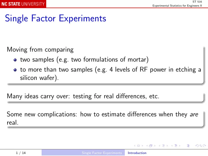
ST 516 Experimental Statistics for Engineers II Single Factor Experiments Moving from comparing two samples (e.g. two formulations of mortar) to more than two samples (e.g. 4 levels of RF power in etching a silicon wafer). Many ideas carry over: testing for real differences, etc. Some new complications: how to estimate differences when they are real. 1 / 14 Single Factor Experiments Introduction

ST 516 Experimental Statistics for Engineers II The data (etch-rate.txt): Power Obs1 Obs2 Obs3 Obs4 Obs5 160 575 542 530 539 570 180 565 593 590 579 610 200 600 651 610 637 629 220 725 700 715 685 710 2 / 14 Single Factor Experiments Example

ST 516 Experimental Statistics for Engineers II Boxplots etchRate <- read.table("data/etch-rate.txt", header = TRUE) etchRateLong <- reshape(etchRate, varying = 2:6, idvar = "Code", v.names = "EtchRate", direction = "long", timevar = "Obs") boxplot(EtchRate ~ Power, etchRateLong, ylab = expression(paste("Rate (", ring(A), "/min)")), xlab = "Power (w)") 3 / 14 Single Factor Experiments Example

ST 516 Experimental Statistics for Engineers II 700 ° /min) 650 Rate (A 600 550 160 180 200 220 Power (w) 4 / 14 Single Factor Experiments Example

ST 516 Experimental Statistics for Engineers II Dot plots plot(EtchRate ~ Power, etchRateLong, ylab = expression(paste("Rate (", ring(A), "/min)")), xlab = "Power (w)") ● ● ● 700 ● ● ° /min) 650 ● ● Rate (A ● ● ● 600 ● ● ● ● ● ● ● 550 ● ● ● 160 170 180 190 200 210 220 Power (w) 5 / 14 Single Factor Experiments Example

ST 516 Experimental Statistics for Engineers II What do we see? Level of power has strong effect. No obvious outliers. Similar spreading at each level. 6 / 14 Single Factor Experiments Example

ST 516 Experimental Statistics for Engineers II Statistical Issues Test whether the observed differences could have been caused by chance (randomization of runs): Null hypothesis H 0 : no difference. If we reject H 0 (and in this example, we expect to!), what differences exist? Point estimates, interval estimates. 7 / 14 Single Factor Experiments Example

ST 516 Experimental Statistics for Engineers II Statistical Models Notation: n replicates for each of a levels of the factor. y i , j = j th response for i th level of factor. The “means” model: y i , j = µ i + ǫ i , j , i = 1 , 2 , . . . , a , j = 1 , 2 , . . . , n . The “effects” model: y i , j = µ + τ i + ǫ i , j , i = 1 , 2 , . . . , a , j = 1 , 2 , . . . , n . 8 / 14 Single Factor Experiments Analysis of Variance

ST 516 Experimental Statistics for Engineers II Broad Approach to Testing Null hypothesis H 0 : means model: µ 1 = µ 2 = · · · = µ a effects model: τ 1 = τ 2 = · · · = τ a = 0 y i · , s 2 Basic summaries: ¯ i , i = 1 , 2 , . . . , a . 9 / 14 Single Factor Experiments Analysis of Variance

ST 516 Experimental Statistics for Engineers II Strategy: reject H 0 if the ¯ y i · ’s differ a lot. We could use max i < i ′ | ¯ y i · − ¯ y i ′ · | . Instead, we effectively use � y i ′ · | 2 . | ¯ y i · − ¯ i < i ′ In either case, we need a denominator to compare with. 10 / 14 Single Factor Experiments Analysis of Variance

ST 516 Experimental Statistics for Engineers II Analysis of Variance (ANOVA) Sums of squares and degrees of freedom ( N = na ): a n a a n � � y ·· ) 2 � y ·· ) 2 � � y i · ) 2 ( y i , j − ¯ = n (¯ y i · − ¯ + ( y i , j − ¯ i =1 j =1 i =1 i =1 j =1 SS Treatments SS Total SS Error df = a − 1 df = N − 1 df = N − a 11 / 14 Single Factor Experiments Analysis of Variance

ST 516 Experimental Statistics for Engineers II For each sum of squares, Sum of Squares Mean Square = degrees of freedom . � y i ′ · | 2 . MS Treatments is proportional to | ¯ y i · − ¯ i < i ′ MS Error is a pooled estimate of common variance σ 2 . 12 / 14 Single Factor Experiments Analysis of Variance

ST 516 Experimental Statistics for Engineers II E(MS Error ) = σ 2 , and � = σ 2 under H 0 E(MS Treatments ) > σ 2 otherwise . As a test statistic, we use F 0 = MS Treatments . MS Error Under H 0 , F 0 is F -distributed with a − 1 and N − a degrees of freedom. 13 / 14 Single Factor Experiments Analysis of Variance

ST 516 Experimental Statistics for Engineers II In R summary(aov(EtchRate ~ factor(Power), data = etchRateLong)) Output Df Sum Sq Mean Sq F value Pr(>F) factor(Power) 3 66871 22290 66.797 2.883e-09 *** Residuals 16 5339 334 --- Signif. codes: 0 *** 0.001 ** 0.01 * 0.05 . 0.1 1 14 / 14 Single Factor Experiments Analysis of Variance