Designed Experiments, One Factor with More Than Two levels The - PowerPoint PPT Presentation

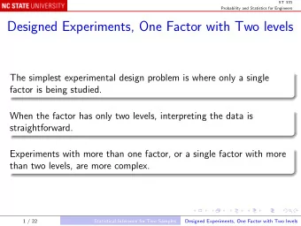
ST 370 Probability and Statistics for Engineers Designed Experiments, One Factor with More Than Two levels The simplest experimental design problem is where only a single factor is being studied. Having more than two levels brings some complications. 1 / 16 One Factor with More Than Two Levels

ST 370 Probability and Statistics for Engineers The tensile strengths for four different compositions of paper are an example of this design: Response: tensile strength; Factor: concentration of hardwood fiber in the pulp; Levels: a = 4 levels: 5%, 10%, 15%, 20%; Replication: n = 6 samples were tested at each level of hardwood concentration. Note Other factors could also affect the tensile strength of the paper: Basis weight; Coatings. These were all held constant . 2 / 16 One Factor with More Than Two Levels Completely Randomized Design

ST 370 Probability and Statistics for Engineers Randomization If feasible, all 24 measurements should be made in random order , in order to prevent drifts in the measurements (caused for example by changing ambient humidity) being confounded with the effect of changing the concentration of hardwood fiber. The design is then called a completely randomized design (CRD). 3 / 16 One Factor with More Than Two Levels Completely Randomized Design

ST 370 Probability and Statistics for Engineers Data Analysis The R tools that we shall use to analyze data collected in factorial experiments are generally: lm() , for fitting l inear m odels; aov() , for the a nalysis o f v ariance. We begin by asking whether the factor had any effect on the response; that is, testing the null hypothesis that it has no effect: H 0 : µ 1 = µ 2 = µ 3 = µ 4 where µ i is the population mean strength for level i , i = 1 , 2 , 3 , 4. 4 / 16 One Factor with More Than Two Levels Completely Randomized Design

ST 370 Probability and Statistics for Engineers For convenience when we use these methods with more than one factor, we write µ i = µ + τ i , i = 1 , 2 , 3 , 4 where: µ is an overall typical value; τ i , called the treatment effect of the i th level, is the deviation of µ i from µ . In terms of these parameters, the null hypothesis is τ 1 = τ 2 = τ 3 = τ 4 . 5 / 16 One Factor with More Than Two Levels Completely Randomized Design

ST 370 Probability and Statistics for Engineers The four parameters µ 1 , µ 2 , µ 3 , and µ 4 have been replaced by five : µ , τ 1 , τ 2 , τ 3 , and τ 4 , which introduces a redundancy. The redundancy is eliminated by imposing a constraint on τ 1 , τ 2 , τ 3 , and τ 4 ; possibilities include: � 4 i =1 τ i = 0, as in the book; τ 4 = 0, as in SAS and JMP; τ 1 = 0, as in R. With the constraint τ 1 = 0, µ 1 = µ + τ 1 = µ, so the “overall typical value” µ is in fact just µ 1 , the mean strength for the first level of the factor, called the baseline (or reference) level. For i � = 1, τ i = µ i − µ = µ i − µ 1 . That is, the i th treatment effect is the difference between the mean strength for level i and for the baseline level. 6 / 16 One Factor with More Than Two Levels Completely Randomized Design

ST 370 Probability and Statistics for Engineers Differences among means Suppose that the sample mean strengths for the 4 levels of hardwood concentration are ¯ y 1 · , ¯ y 2 · , ¯ y 3 · , and ¯ y 4 · , respectively: n y i · = 1 � ¯ y i , j n j =1 where y i , j is the j th measurement for the i th level of hardwood concentration. To test the null hypothesis, we need a measure of how different these means are. 7 / 16 One Factor with More Than Two Levels Completely Randomized Design

ST 370 Probability and Statistics for Engineers With only two levels, this was easy: | ˆ δ | = | ¯ y 2 · − ¯ y 1 · | is the obvious choice; with more than two levels, various measures could be used: The range , max i , i ′ | ¯ y i · − ¯ y i ′ · | ; The sum , � i , i ′ | ¯ y i · − ¯ y i ′ · | ; y i ′ · | 2 . The sum of squares , � i , i ′ | ¯ y i · − ¯ The first measure, the range, is important, but the conventional measure is the third, in the form of the Treatment sum of squares : a � y ·· ) 2 . SS Treatments = n (¯ y i · − ¯ i =1 8 / 16 One Factor with More Than Two Levels Completely Randomized Design

ST 370 Probability and Statistics for Engineers When there are two levels, we standardize | ˆ δ | = | ¯ y 2 · − ¯ y 1 · | by dividing by its standard error, to form the t -statistic. Now, with more than two levels, we also need to form a ratio, the F -statistic: MS Treatments = SS Treatments a − 1 a n � � y i · ) 2 SS Errors = ( y i , j − ¯ i =1 j =1 MS Errors = SS Errors a ( n − 1) F obs = MS Treatments MS Errors 9 / 16 One Factor with More Than Two Levels Completely Randomized Design

ST 370 Probability and Statistics for Engineers The ANOVA table The calculations are usually laid out in a table: Source Degrees Sum Mean F -ratio of Freedom of Squares Square Treatments a − 1 SS Treatments MS Treatments F obs Errors a ( n − 1) SS Errors MS Errors Total an − 1 SS Total The sums of squares are related by the Analysis of Variance (ANOVA) equation: a n y ·· ) 2 = SS Treatments + SS Errors � � SS Total = ( y i , j − ¯ i =1 j =1 10 / 16 One Factor with More Than Two Levels Completely Randomized Design

ST 370 Probability and Statistics for Engineers Finding the P -value When we measure the extent of the differences among ¯ y 1 · , ¯ y 2 · , ¯ y 3 · , and ¯ y 4 · by the F -ratio, we still need to find the probability of obtaining as large a value as F obs , when the null hypothesis H 0 : τ 1 = τ 2 = τ 3 = τ 4 = 0 is true. As before, we assume that the measurements follow the normal distribution with the same standard deviation, and then it can be shown that, when the null hypothesis is true, F follows a related distribution called Snedecor’s (or Fisher’s) F -distribution. The probability that F ≥ F obs can be calculated as an area under the corresponding density function. 11 / 16 One Factor with More Than Two Levels Completely Randomized Design

ST 370 Probability and Statistics for Engineers In R summary(aov(Strength ~ factor(Hardwood), paper)) # output: # Df Sum Sq Mean Sq F value Pr(>F) # factor(Hardwood) 3 382.8 127.60 19.61 3.59e-06 *** # Residuals 20 130.2 6.51 # --- # Signif. codes: 0 *** 0.001 ** 0.01 * 0.05 . 0.1 1 The P -value is extremely small: we have strong evidence that the null hypothesis should be rejected. 12 / 16 One Factor with More Than Two Levels Completely Randomized Design

ST 370 Probability and Statistics for Engineers Comparing the sample means When, as in the paper example, we reject the null hypothesis of no effect: H 0 : τ 1 = τ 2 = τ 3 = τ 4 = 0 , the next question is: what is the effect? For instance: which levels of hardwood concentration give significantly higher tensile strength than other levels? We can answer this question either: one pair of levels at a time; for all pairs simultaneously. 13 / 16 One Factor with More Than Two Levels Comparing Means

ST 370 Probability and Statistics for Engineers One pair at a time For a given pair of means, say µ 1 and µ 2 , we could test the null hypothesis H 0;1 , 2 : µ 1 = µ 2 in the same way as when there were only two levels: y 1 · − ¯ ¯ y 2 · t obs:1 , 2 = standard error where � 1 � + 1 � standard error = MS E . n 1 n 2 Note that MS E replaces s 2 pooled ; in fact, when a = 2, they are the same. 14 / 16 One Factor with More Than Two Levels Comparing Means

ST 370 Probability and Statistics for Engineers We reject H 0: i , i ′ when | t obs: i , i ′ | ≥ t . 025 , 20 . For the paper strength data, we reject all the null hypotheses except H 0:2 , 3 . That is, we cannot state that strength of 10% hardwood paper is significantly different from that of 15% hardwood paper, but all other differences are significant. 15 / 16 One Factor with More Than Two Levels Comparing Means

ST 370 Probability and Statistics for Engineers Equivalently, we could calculate confidence intervals for each pairwise difference µ i − µ i ′ . The null hypothesis H 0: i , i ′ is rejected if and only if the confidence interval does not contain zero. Each confidence interval is of the form y i · − ¯ ¯ y i ′ · ± LSD where LSD is Fisher’s Least Significant Difference: � 1 � + 1 � LSD = t . 025 , 20 MS E = 3 . 07 . n i n i ′ 16 / 16 One Factor with More Than Two Levels Comparing Means