Simple Linear Regression and Correlation Model for designed - PowerPoint PPT Presentation

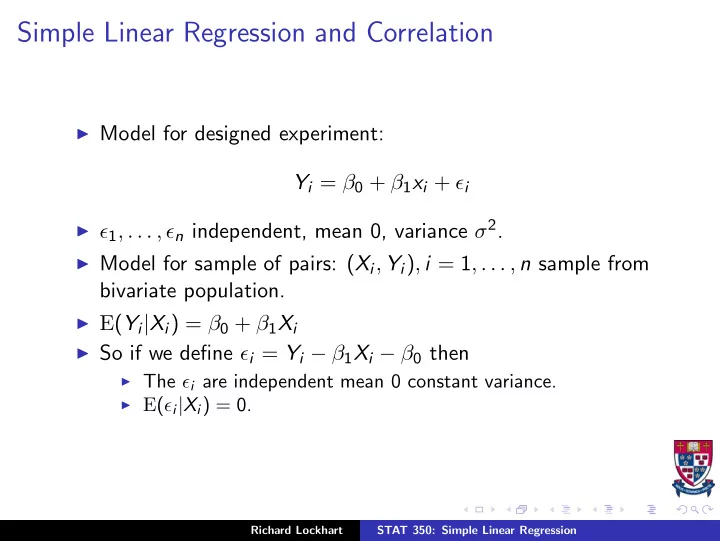
Simple Linear Regression and Correlation ◮ Model for designed experiment: Y i = β 0 + β 1 x i + ǫ i ◮ ǫ 1 , . . . , ǫ n independent, mean 0, variance σ 2 . ◮ Model for sample of pairs: ( X i , Y i ) , i = 1 , . . . , n sample from bivariate population. ◮ E ( Y i | X i ) = β 0 + β 1 X i ◮ So if we define ǫ i = Y i − β 1 X i − β 0 then ◮ The ǫ i are independent mean 0 constant variance. ◮ E ( ǫ i | X i ) = 0. Richard Lockhart STAT 350: Simple Linear Regression

Bivariate Normal Populations ◮ X , Y have a bivariate normal distribution if they have joint density 1 − q ( x , y ) / { 2(1 − ρ 2 ) } � � f ( x , y ) = 1 − ρ 2 exp � σ 1 σ 2 where q ( x , y ) = ( x − µ 1 ) 2 + ( y − µ 2 ) 2 − 2 ρ ( x − µ 1 ) ( y − µ 2 ) σ 2 σ 2 σ 1 σ 2 1 2 ◮ Marginal density of X is N ( µ 1 , σ 2 1 ). ◮ Marginal density of Y is N ( µ 2 , σ 2 1 ). Richard Lockhart STAT 350: Simple Linear Regression

◮ This is a density if − 1 < ρ < 1 and σ 1 , σ 2 are both positive. ◮ Covariance of X and Y is E { ( X − µ 1 )( Y − µ 2 ) } = ρσ 1 σ 2 ◮ The correlation coefficient is ρ ; that is � ( X − µ 1 ) � ( Y − µ 2 ) = ρ E σ 1 σ 2 ◮ Conditional distribution of Y given X = x is Normal, mean x − µ 1 β 0 + β 1 x = µ 2 + ρσ 2 σ 1 and variance σ 2 = (1 − ρ ) 2 σ 2 2 . Richard Lockhart STAT 350: Simple Linear Regression

Estimation of parameters ◮ The population means are estimated by sample means: µ 1 = ¯ µ 2 = ¯ ˆ ˆ X Y ◮ Population SDs are estimated by sample SDs: �� �� i ( X i − ¯ i ( Y i − ¯ X ) 2 Y ) 2 σ 1 ≡ s x = ˆ σ 2 ≡ s y = ˆ n − 1 n − 1 ◮ Population correlation estimated by sample correlation: i ( X i − ¯ X )( Y i − ¯ P Y ) n − 1 ρ ≡ r = ˆ s x s y Richard Lockhart STAT 350: Simple Linear Regression

Estimation with fixed covariates ◮ Ordinary least squares estimate of slope β 1 is i ( X i − ¯ X )( Y i − ¯ � Y ) β 1 = r s y ˆ = i ( Y i − ¯ s x � Y ) 2 ◮ Ordinary least squares estimate of intercept β 0 is β 0 = ¯ ˆ Y − ˆ β 1 ¯ X . ◮ Ordinary least squares estimate of σ 2 is residual mean square: σ 2 = � ( Y 1 − ˆ β 0 − ˆ β 1 X i ) 2 / ( n − 2) . ˆ i ◮ This estimate is unbiased: σ 2 ) = σ 2 . E (ˆ Richard Lockhart STAT 350: Simple Linear Regression

Relation between the models ◮ In both models Var ( ǫ i ) = σ 2 . ◮ In bivariate normal model Var ( ǫ i ) = σ 2 = σ 2 y (1 − ρ 2 ) . Richard Lockhart STAT 350: Simple Linear Regression

Simple linear regression: least squares, inference ◮ See Fitting Linear Models lecture for derivation of least squares formulas. ◮ The estimates ˆ β 1 and ˆ β 2 are linear combinations of the Y i . For instance ˆ � β 1 = w i Y i where x i − ¯ x w i = x ) 2 . � i ( x i − ¯ ◮ So E (ˆ � � β 1 ) = w i E ( Y i ) = w i ( β 0 + β 1 x i ) i i � = 0 + β 1 w i x i i = β 1 Richard Lockhart STAT 350: Simple Linear Regression

◮ Notice use of fact that � w i = 0 so � w i ¯ X = 0. ◮ The identity says ˆ β 1 is an unbiased estimate of β 1 . ◮ We can compute the variance: � � w 2 Var ( w i Y i ) = i Var ( Y i ) i i x ) 2 � ( x i − ¯ = σ 2 x ) 2 } 2 { � ( x i − ¯ σ 2 = � ( x i − ¯ x ) 2 ◮ The square root of the variance of any estimate is called its Standard Error . Richard Lockhart STAT 350: Simple Linear Regression

Distribution Theory ◮ Both ˆ β 1 and ˆ β 2 are linear combinations of the normally distributed Y i . ◮ So both have normal distributions. ◮ So you can form confidence intervals: ˆ β i ± t n ,α/ 2 Estimated Standard Error ◮ and test hypotheses using ˆ β i − β i , o t = Estimated Standard Error ◮ ESE is theoretical SE with σ estimated. ◮ Use residual mean square to estimate σ 2 . Richard Lockhart STAT 350: Simple Linear Regression

Output from JMP R Square 0.534338 Root Mean Square Error 1.96287 Mean of Response 32.44423 Estimates Term Estimate Std Error t Ratio Prob>|t| Intercept 11.098156 1.953928 5.68 <.0001 Distance 0.0481812 0.004389 10.98 <.0001 Can form CIs and test hypotheses like H o : β 1 = 0. Richard Lockhart STAT 350: Simple Linear Regression

Output from JMP Analysis of Variance Source DF Sum of Squares Mean Square F Ratio Model 1 464.21357 464.214 120.4855 Error 105 404.55022 3.853 Prob > F C. Total 106 868.76379 <.0001 Notice F = t 2 , that is 120 . 4855 = 10 . 98 2 . Always happens with 1 df F -test. Richard Lockhart STAT 350: Simple Linear Regression