Shape Correspondence and Functional Maps SGP 2017 course Maks - PowerPoint PPT Presentation
Shape Correspondence and Functional Maps SGP 2017 course Maks Ovsjanikov Based on joint work with: E. Corman, A. Chambolle, M. Ben-Chen, O. Azencot, A. Butscher, R. Rustamov, J. Solomon, F. Chazal, L. Guibas, D. Nogneng, . Laboratoire
Shape Correspondence and Functional Maps SGP 2017 course Maks Ovsjanikov Based on joint work with: E. Corman, A. Chambolle, M. Ben-Chen, O. Azencot, A. Butscher, R. Rustamov, J. Solomon, F. Chazal, L. Guibas, D. Nogneng, …. Laboratoire d’Informatique de l’École polytechnique
General Overview Overall Objective : Create tools for computing and analyzing mappings between geometric objects.
General Overview Overall Objective : Create tools for computing and analyzing mappings between geometric objects. Rather than comparing points on objects it is often easier to compare real-valued functions defined on them. Such maps can be represented as matrices.
Course Overview [Related] Course Website: http://www.lix.polytechnique.fr/~maks/fmaps_course/ or http://bit.do/fmaps Course Notes: Linked from the website. Or use: http://bit.do/fmaps_notes Sample Code: See Sample Code link on the website.
Course Overview Motivation and Problem Taxonomy Rigid Matching: ICP Functional Map representation, properties Basic pipeline for non-rigid matching Extensions, Improvements Open problems, Q&A
What is a Shape? Continuous: a surface embedded in 3D. Discrete: a graph embedded in 3D (triangle mesh). Common assumptions: • Connected. • Manifold. • Without Boundary.
What is a Shape? Continuous: a surface embedded in 3D. Discrete: a graph embedded in 3D (triangle mesh). 5k – 200k triangles Shapes from the FAUST, SCAPE, and TOSCA datasets
Overall Goal Given two shapes, find correspondences between them.
Overall Goal Given two shapes, find correspondences between them. Finding the best map between a pair of shapes.
Problem Taxonomy Local vs. Global refinement (e.g. ICP) | alignment (search) . . Rigid vs. Deformable rotation, translation | general deformation. Semi vs. Fully Automatic given landmarks | a priori model Learning-Based vs. Direct known examples | unseen data
Problem Taxonomy Local vs. Global refinement (e.g. ICP) | alignment (search) . . Rigid vs. Deformable rotation, translation | general deformation. Semi vs. Fully Automatic given landmarks | a priori model Learning-Based vs. Direct known examples | unseen data
Why Shape Matching? Given a correspondence, we can transfer: texture and parametrization segmentation and labels deformation Sumner et al. ‘04. Other applications: shape interpolation, reconstruction ... 12
Rigid Shape Matching • Given a pair of shapes, find the optimal Rigid Alignment between them. • The unknowns are the rotation/translation parameters of the source onto the target shape.
Iterative Closest Point (ICP) • Classical approach: iterate between finding correspondences and finding the transformation: example in 2D N M Given a pair of shapes, and , iterate: N M 1. For each find nearest neighbor . y i ∈ N x i ∈ M 2. Find optimal transformation minimizing: X k Rx i + t � y i k 2 arg min 2 R,t i
Iterative Closest Point • Classical approach: iterate between finding correspondences and finding the transformation: N M Given a pair of shapes, and , iterate: N M 1. For each find nearest neighbor . y i ∈ N x i ∈ M 2. Find optimal transformation minimizing: X k Rx i + t � y i k 2 arg min 2 R,t i
Iterative Closest Point • Classical approach: iterate between finding correspondences and finding the transformation: N M Given a pair of shapes, and , iterate: N M 1. For each find nearest neighbor . y i ∈ N x i ∈ M 2. Find optimal transformation minimizing: X k Rx i + t � y i k 2 arg min 2 R,t i
Iterative Closest Point • Classical approach: iterate between finding correspondences and finding the transformation: N M Given a pair of shapes, and , iterate: N M 1. For each find nearest neighbor . y i ∈ N x i ∈ M 2. Find optimal transformation minimizing: X k Rx i + t � y i k 2 arg min 2 R,t i
Iterative Closest Point • Classical approach: iterate between finding correspondences and finding the transformation: N M Given a pair of shapes, and , iterate: N M 1. For each find nearest neighbor . y i ∈ N x i ∈ M 2. Find optimal transformation minimizing: X k Rx i + t � y i k 2 arg min 2 R,t i
Iterative Closest Point • Classical approach: iterate between finding correspondences and finding the transformation: N M Given a pair of shapes, and , iterate: N M 1. For each find nearest neighbor . y i ∈ N x i ∈ M 2. Find optimal transformation minimizing: X k Rx i + t � y i k 2 arg min 2 R,t i
Iterative Closest Point • Classical approach: iterate between finding correspondences and finding the transformation: N M Given a pair of shapes, and , iterate: N M 1. For each find nearest neighbor . y i ∈ N x i ∈ M 2. Find optimal transformation minimizing: X k Rx i + t � y i k 2 arg min 2 R,t i
Iterative Closest Point • Classical approach: iterate between finding correspondences and finding the transformation: N M 1. Finding nearest neighbors: can be done with space- partitioning data structures (e.g., KD-tree). 2. Finding the optimal transformation minimizing: X k Rx i + t � y i k 2 arg min 2 R,t i Arun et al., Least- Can be done efficiently via SVD decomposition. Squares Fitting of Two 3-D Point Sets
ICP: Optimal Transformation Problem Formulation: 1. Given two sets points: in . Find the rigid transform: { x i } , { y i } , i = 1 ..n N that minimizes: R , t X k R x i + t � y i k 2 2 i =1 2. Closed form solution: 1. Construct: , where i =1 ( y i − µ Y )( x i − µ X ) T C = P N µ X = 1 P i x i , µ N 2. Compute the SVD of C: C = U Σ V T , µ Y = 1 P i y i , N det( UV T ) = 1 , R opt = UV T 1. If R opt = U ˜ Σ V T , ˜ 2. Else Σ = diag(1 , 1 , . . . , − 1) 3. Set t opt = µ Y − R opt µ X Note that C is a 3x3 matrix. SVD is very fast. Arun et al., Least-Squares Fitting of Two 3-D Point Sets
Non-Rigid Shape Matching Unlike rigid matching with rotation/translation, there is no compact representation to optimize for in non-rigid matching.
Non-Rigid Shape Matching Main Problems: • What does it mean for a correspondence to be “good”? • How to compute it efficiently in practice?
Isometric Shape Matching Possible Model: Good maps must preserve geodesic distances. N d N ( T ( x ) , T ( y )) d M ( x, y ) M Geodesic: length of shortest path lying entirely on the surface.
Isometric Shape Matching Approach: N d N ( T ( x ) , T ( y )) d M ( x, y ) M Find the point mapping by minimizing the distance distortion: k d M ( x, y ) � d N ( T ( x ) , T ( y )) k X T opt = arg min T x,y The unknowns are point correspondences.
Isometric Shape Matching Approach: N d N ( T ( x ) , T ( y )) d M ( x, y ) M Find the point mapping by minimizing the distance distortion: k d M ( x, y ) � d N ( T ( x ) , T ( y )) k X T opt = arg min T x,y Problem: The space of possible solutions is highly non-linear, non-convex.
Functional Map Representation We would like to define a representation of shape maps that is more amenable to direct optimization. 1. A compact representation for “natural” maps. 2. Inherently global and multi-scale. 3. Handles uncertainty and ambiguity gracefully. 4. Allows efficient manipulations (averaging, composition). 5. Leads to simple (linear) optimization problems.
Background: Laplace-Beltrami Operator Given a compact Riemannian manifold without M boundary, the Laplace-Beltrami operator : ∆ ∆ : C ∞ ( M ) ! C ∞ ( M ) , ∆ f = div r f
Heat Equation on a Surface Given a compact surface without boundary the evolution of heat is given by: ∂ f ∂ t = ∆ f = div r f.
Laplace-Beltrami Operator Given a compact surface without boundary, M the Laplace-Beltrami operator : ∆ 1. Is invariant under isometric deformations. 2. Has a countable eigendecomposition: ∆ φ i = λ i φ i L 2 ( M ) that forms an orthonormal basis for . 3. Characterizes the geodesic distances fully.
Laplace-Beltrami Eigenfunctions The Laplace-Beltrami operator has an ∆ eigendecomposition: ∆ φ i = λ i φ i φ 3 φ 0 φ 1 φ 2 . . . λ 0 = 0 λ 1 = 2 . 6 λ 2 = 3 . 4 λ 3 = 5 . 1 Ordered from low frequency (smoothest) to higher frequency (oscillating). Z kr φ i ( x ) k 2 dµ ( x ) λ i = M
Laplace-Beltrami Eigenfunctions L 2 ( M ) …. that forms an orthonormal basis for : Any (square-integrable) can be represented f : M → R as a linear combination of the LB eigenfunctions. a 0 + a 1 + = . . . φ 0 φ 1 ∞ Z X a i = f ( x ) φ i ( x ) dµ ( x ) f = a i φ i M i =0
In the Discrete World • Functions are defined at vertices of the mesh. • Integration is defined with respect to a discrete volume measure: 2 = f T Af k f k 2 - diagonal matrix of area weights. A • Laplacian is discretized as a matrix L = A − 1 W i 1 L ij = 2 A ( j ) (cot( α ij ) + cot( β ij )) t 1 t 2 α ij β ij Can be derived from 1 st order FEM. j
Recommend
More recommend
Explore More Topics
Stay informed with curated content and fresh updates.
