Session 5 A brief introduction to Predictive Modeling Lichen Bao, - PDF document
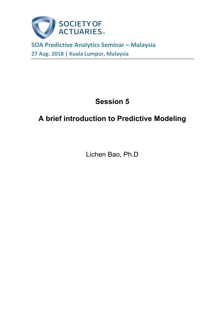
SOA Predictive Analytics Seminar Malaysia 27 Aug. 2018 | Kuala Lumpur, Malaysia Session 5 A brief introduction to Predictive Modeling Lichen Bao, Ph.D A Brief Introduction to Predictive Modeling LICHEN BAO Data Scientist, RGA Reinsurance
SOA Predictive Analytics Seminar – Malaysia 27 Aug. 2018 | Kuala Lumpur, Malaysia Session 5 A brief introduction to Predictive Modeling Lichen Bao, Ph.D
A Brief Introduction to Predictive Modeling LICHEN BAO Data Scientist, RGA Reinsurance Company August 27, 2018
Agenda • Overview of Predictive Modeling (PM) • A Case Study • PM for Actuaries
Overview of Predictive Modeling (PM)
What is Predictive Modeling? Modeling covers the statistics models and algorithms. Data High quality data Modeling Modeling Statistical model Statistical model Prediction Business decisions 4
Review of Predictive Modeling Linear regression and OLS may sound familiar … Linear regression model • Y target/response variable; X i explanatory/predictor variable • β i parameters to be estimated • ε error term/noise Underlying Assumptions for a Valid LM • Normality, 𝜁 ~ N ( 0,σ 2 ) • Linearity; Homogeneity- Y for population; Fixed X , error-free; Observation independence 5
Review of Predictive Modeling Linear regression and OLS may sound familiar … Ordinary Least Squares(OLS) 𝑧 𝑗 − 𝑧 𝑗 ) 2 = 𝑏𝑠 min 𝑗 ( 𝑘 𝛾 𝑘 𝑌 𝑗𝑘 − 𝑧 𝑗 ) 2 β = 𝑏𝑠 min 𝑆𝑇𝑇 = 𝑏𝑠 min 𝑗 ( • For a simple regression 2 − 1 ( 𝑦 𝑗 𝑧 𝑗 − 1 𝑜 𝑦 𝑗 𝑧 𝑗 ) ( 𝑦 𝑗 𝑜 ( 𝑦 𝑗 ) 2 ) , 𝑧 − β 1 = β 0 = β 1 𝑦 Identical to Maximum likelihood estimator More robust and consistent approach β = 𝑏𝑠 m𝑏𝑦 𝑀(𝑌, 𝑍, 𝛾) = 𝑏𝑠 min −ln(𝑀 𝑌, 𝑍, 𝛾 ) = 𝑏𝑠 min 𝑗 (𝑧 𝑗 − 𝑧 𝑗 (𝜈 𝑗 )) 2 if normal distribution Use adj R 2 to compare fitness of models • 1 = 𝑆𝑇𝑇 𝑈𝑇𝑇 + 𝐹𝑇𝑇 portion that has been explained by OLS model • portion of TSS for the error 𝑈𝑇𝑇 𝑍𝑗)2 Define 𝑆 2 = 𝑆𝑇𝑇 𝑗(𝑍𝑗− 𝑈𝑇𝑇 = 1 − 𝐹𝑇𝑇 𝑈𝑇𝑇 = 𝑍)2 , but it is biased 𝑗(𝑍𝑗− Adjusted 𝑆 2 = 1 − 𝐹𝑇𝑇 𝑈𝑇𝑇 ∗ 𝑜−1 𝑜−𝑙 = 1 − (1−𝑆 2 ) ∗ 𝑜−1 𝑜−𝑙 6
Review of Predictive Modeling We barely see any real application of OLS in life insurance because of the constraints. Features of OLS Applications in Insurance Binomial for rate Validation of assumptions - (mortality/lapse/UW, etc.), σ 2 Normal w/ constant σ 2 ~ r(1-r) × Poisson for claim count, ~ Non-linear relationship, mean esp. for extrapolation Unmatched Gamma for claim amount, ~ Unbounded data, non- mean 2 negative value 7
Generalized Linear Model (GLM) GLM is extensively used in insurance industry. Includes most Major focus of PM in distributions related to insurance industry insurance OLS model is a special Great flexibility in case of GLM variance structure (Relatively) Easy to Multiplicative model understand and intuitive & consistent communicate with insurance practice 8
Generalized Linear Model (GLM) GLM is extensively used in insurance industry. Random component Systematic component Link function 9
Generalized Linear Model (GLM) GLM is extensively used in insurance industry. Random component Observations Y 1 , . . . , Y n are independent w/ density from the exponential family 𝑗 𝑧 𝑗 ; 𝜄 𝑗 , = 𝑓𝑦𝑞 𝑧 𝑗 𝜄 𝑗 − 𝑐(𝜄 𝑗 ) + 𝑑(𝑧 𝑗 , ) 𝑔 𝑏 𝑗 ( ) From maximum likelihood theory, 𝐹 𝑍 = 𝜈 = 𝑐 ′ 𝜄 , 𝑤𝑏𝑠 𝑍 = 𝑐 ′′ 𝜄 𝑏 = 𝑏 𝑊(𝜈) Each distribution is specified in terms of mean & variance Variance is a function of mean Norm ormal al Poiss oisson Bin inomial Gam amma InverseGauss ssian 𝑂(𝜈, 2 ) 𝐻(𝜈, ) 𝐽𝐻(𝜈, 2 ) Name 𝑄(𝜈) 𝐶(𝑛, 𝜌) 𝑛 (- ,+ ) (0,+ ) (0,+ ) (0,+ ) Range (0,1) ln(1+e ) e 2 −(−2𝜄) 1/2 b(𝜄) − ln −𝜄 e e / (1+e ) (−2𝜄) −1/2 𝜈(𝜄) 𝜄 − 1/ 𝜄 𝜈 2 𝜈 3 𝑊(𝜈) 𝜈 𝜈(1 − 𝜈) 1 10
Generalized Linear Model (GLM) GLM is extensively used in insurance industry. Systematic component A linear predictor 𝑗 = 𝑘 𝑦 𝑗𝑘 𝛾 𝑘 = 𝑌𝛾 for observation i link function 𝑗 = (𝜈 𝑗 ) , random & systematic are connected by a smooth & invertible function Ide dentity Log Log Logit Log Rec eciprocal 𝑦 (𝜈 𝑗 ) 𝑦 ln(𝑦) 1/𝑦 ln( 1 − 𝑦) −1 ( 𝑗 ) 𝑓 𝑦 𝑓 𝑦 𝑦 1/𝑦 1+𝑓 𝑦 Log is unique in insurance application s.t. all parameters are multiplicative 𝑦 𝑗𝑘 = 𝑘 𝑔 𝑦 𝑗𝑘 𝑧 = exp( 𝑘 𝑦 𝑗𝑘 𝛾 𝑘 ) = 𝑘 exp 𝑦 𝑗𝑘 𝛾 𝑘 = 𝑘 exp 𝛾 𝑘 𝑘 Consistent with most insurance practices Intuitively easy to understand and communicate 11
Generalized Linear Model (GLM) GLM is extensively used in insurance industry. Comparison with OLS Random Systematic Link 𝐹 𝑧 𝑗 = 𝑗 OLS Normal only 𝑗 = 𝑦 𝑗𝑘 𝛾 𝑘 𝐹(𝑧 𝑗 ) = 𝑗 GLM Various distribution 𝑘 Inclusion of most distributions related to insurance data • Normal, binomial, Poisson, Gamma, inverse-Gaussian, Tweedie Link function Application sample Normal General Application Poisson Claim frequency, counts Bernoulli Retention, cross-sell, underwriting rates Negative Binomial Claim severity Gamma Claim severity Tweedie Claim cost Inverse Gaussian Claim severity 12
An Inventory of the Methods There are plenty of statistical modeling methods out there. Random Forest XG-boost machine Gradient Boosting Support vector machine Ada Boosting Survey Data Analysis Ensemble method Sentiment Analysis Genetic Algorithms Markov chain Monte Carlo Bayesian Analysis Optimization Methods Decision Trees Feature engineering Neural Networks / Deep learning Analysis of Variance Classification/Association Categorical Data Analysis Mixed Models Survival Analysis Multivariate Analysis Non-Parametric Analysis Cluster Analysis Text mining Machine Learning & Statistical Techniques
Predictive Modeling by Classes There are different terminologies regarding predictive modeling. Supervised vs. Classification vs. Parametric vs. Non- Unsupervised Learning Regression Parametric • Parametric Statistics: • Supervised: estimate • Classification: to expected value of Y segment observations probabilistic model of data given values of X . into 2 or more GLM, Cox, CART, categories. Fraud vs. Poisson Regression(claims MARS, Random legitimate, lapsed vs. count), Gamma (claim Forests, SVM, NN, retained, UW class amount) etc. • Regression: to predict • Unsupervised: find a continuous amount. • Non-Parametric Statistics: no interesting patterns Dollars of loss for a probability model amongst X; no target policy, ultimate size of specified variable Y claim Classification trees, Cl ustering, NN Correlation / Principal Components / Factor Analysis 14
Choosing the Right Method There is always the trade-off between interpretability and flexibility. Trade-Off Between Interpretability and Flexibility Decision Trees GLM Models Interpretability • Logistic Regression Often referred to as simple, • Poisson Regression transparent models Gradient Boosted Often referred to as “machine Trees learning”, black-box models Random Forest Flexibility This is just a sample of many algorithms available 15
Choosing the Right Method There is always the trade-off between interpretability and flexibility. Interpretability Flexibility “Transparent” Algorithms “Black-box” Algorithms More human intervention Less human intervention More interpretable Less interpretable Require more data Require less data Faster to estimate a model Slower to estimate a model Good at handling smooth effects (e.g., Not good at handling smooth effects (e.g., age, income, etc.) age, income, etc.) The model we choose might not be a Higher predictive accuracy because good match to reality, resulting in poor functional form is derived from the data, predictions. not assumed. Less likely to overfit the data More likely to overfit the data 16
Choosing the Right Method Choosing the right algorithm is a combination of statistical and business considerations. Business Considerations Statistical Considerations Experience Dependent Variable Some business problems are well-defined and are Knowing whether the dependent variable is available (or historically modeled a specific way successfully. not), if available whether its continuous, binary, or a Example: Poisson Regression for Experience count helps us narrow down the appropriate algorithm. Studies Know your audience Amount of Data The successful business implementation of a Powerful algorithms (e.g., random forest) require more model may require buy-in from many different data to work well. groups throughout an organization. Model interpretability may be critical, particularly for analyzing experience study data . Model Validation Data Scientists build many models, and pick the Technical Implementation champion model based on which model predicts new Sometimes the increased accuracy in more data the best (e.g., higher accuracy) complex models doesn’t warrant the additional technical difficulties. 17
A Case Study
Recommend
More recommend
Explore More Topics
Stay informed with curated content and fresh updates.
