Sequential Monte Carlo Methods Click to edit Master text styles - PowerPoint PPT Presentation

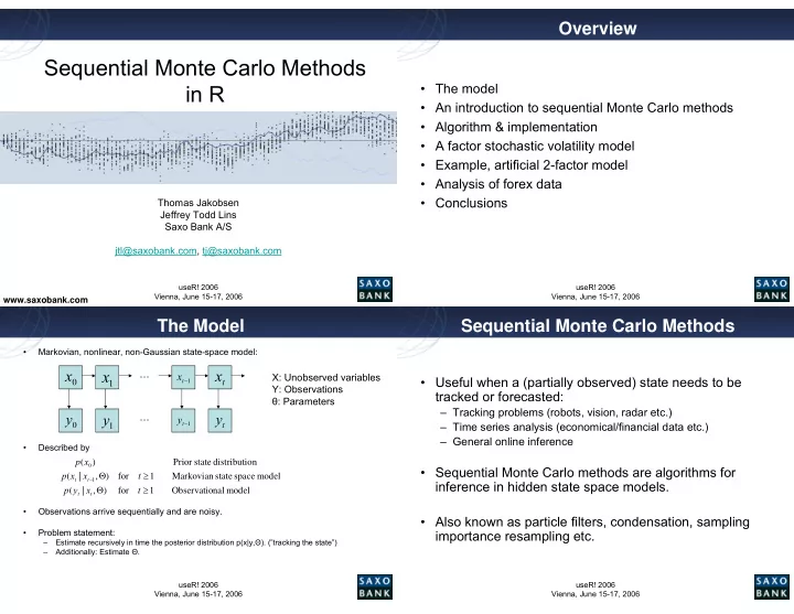
Overview Sequential Monte Carlo Methods • Click to edit Master text styles • Click to edit Master text styles in R • The model • An introduction to sequential Monte Carlo methods • Second level • Second level • Algorithm & implementation • Third level • Third level • A factor stochastic volatility model • Fourth level • Fourth level • Example, artificial 2-factor model • Analysis of forex data • Fifth level • Fifth level • Conclusions Thomas Jakobsen Jeffrey Todd Lins Saxo Bank A/S jtl@saxobank.com, tj@saxobank.com useR! 2006 useR! 2006 Vienna, June 15-17, 2006 Vienna, June 15-17, 2006 www.saxobank.com The Model Sequential Monte Carlo Methods • Markovian, nonlinear, non-Gaussian state-space model: x x x … x X: Unobserved variables • Click to edit Master text styles • Useful when a (partially observed) state needs to be • Click to edit Master text styles − t t 0 1 1 Y: Observations tracked or forecasted: θ : Parameters • Second level • Second level – Tracking problems (robots, vision, radar etc.) y y … y y − t t – Time series analysis (economical/financial data etc.) 0 1 1 • Third level • Third level – General online inference • Described by • Fourth level • Fourth level p x ( ) Prior state distributi on 0 • Sequential Monte Carlo methods are algorithms for Θ ≥ p x x t ( | , ) for 1 Markovian state space model − t t • Fifth level 1 • Fifth level inference in hidden state space models. Θ ≥ p y x t ( | , ) for 1 Observatio nal model t t • Observations arrive sequentially and are noisy. • Also known as particle filters, condensation, sampling • Problem statement: importance resampling etc. – Estimate recursively in time the posterior distribution p(x|y, Θ ). (”tracking the state”) – Additionally: Estimate Θ . useR! 2006 useR! 2006 Vienna, June 15-17, 2006 Vienna, June 15-17, 2006

Sequential Monte Carlo Methods A bootstrap approach (from [1]) Unweighted measure • SMC methods: Basically a nonlinear, non-Gaussian • Click to edit Master text styles • Click to edit Master text styles version of the Kalman filter (but approximate – not closed form) • Second level • Second level Compute importance weights using info at time t-1 • Third level • Third level • The posterior at time t-1 is represented by a set of Weighted measure weighted particles. The particles are drawn i.i.d. and • Fourth level • Fourth level Resampling recursively updated. • Fifth level • Fifth level • Next slide: Illustration of update Prediction Apprx. of p(x_t|y_1:t-1) useR! 2006 useR! 2006 Vienna, June 15-17, 2006 Vienna, June 15-17, 2006 Comb. Parameter and State Estimation Algorithm • Liu & West, Combined Parameter and State Estimation: (auxiliary particle filter with state estimation) • Click to edit Master text styles • Click to edit Master text styles • Often the parameters are known (or obtained through j Θ j j = x ( ) ( ) w ( ) j N Input : Monte Carlo sample ( , ) and weights , 1 ,..., . separate analysis). t t t = µ j = j Θ j • Second level • Second level j N ( ) E x x ( ) ( ) 1. For 1 ,..., : ( | , ) + + t 1 t 1 t t ∈ k 2. Sample an integer {1,..., N} with probabilit y • However: If parameters are unknown, how to carry out • Third level • Third level combined estimation of x and Θ ? j ∝ j µ j j g ( ) w ( ) p y ( ) m ( ) ( | , ) t + t t + t + t 1 1 1 Θ k ⋅ k ( ) N m ( ) h 2 V • Fourth level • Fourth level 3 . Sample ~ ( | , ). + t t t 1 • Liu & West describe a simple approach. ⋅ Θ x k p x k k ( ) ( ) ( ) 4 . Sample ~ ( | , ). + t t t 1 • Fifth level • Fifth level Θ k k p y x ( ) ( ) ( | , ) k ∝ + + + w ( ) t t t 1 1 1 5 . Evaluate weight : + t µ 1 p y ( k ) m ( k ) ( | , ) + + t t t 1 1 Repeat 2. - 5. until approximat ion is sufficient ly accurate. = Θ j + − Θ (j) a ( ) a m ( 1 ) t t t Θ Θ j j V ( ) w ( ) , : Posterior mean and variance matrix from and weights t t t t useR! 2006 useR! 2006 Vienna, June 15-17, 2006 Vienna, June 15-17, 2006

R Implementation Factor Stochastic Volatility Model • To describe the model, the user supplies his own • (similar to the model of Liu & West) functions as arguments to main SMC function (together • Click to edit Master text styles • Click to edit Master text styles with Y and [hyper]parameters). = + + y α Xf ε Observatio ns t t t t α • Second level • Second level Local series level t • R language very suitable for implementation, X Factor loadings matrix • Third level • Third level especially because of ⋅ f N H ~ ( | 0 , ) Factors t t – Vectorization = Κ H h h diag ( , , ) Factor var iances • Fourth level • Fourth level t t tk 1 – Built-in statistical functions = h λ exp( ) ti ti – The possibility of supplying user-defined functions as arguments = + − + • Fifth level • Fifth level λ µ Φ λ µ γ ( ) Log factor var iances − t t t 1 – Ease of visualization and interaction γ ⋅ N 0, U ~ ( | ) Innovation s t U Innovation s variance matrix • Quite efficient but still computationally heavy. ⋅ ε N 0, Ψ ~ ( | ) Idiosyncra tic noise variances t = Ψ Ψ Ψ – For large datasets, a C/C++ optimization is needed diag( ,..., ) 1 k (we already developed a faster C# version). useR! 2006 useR! 2006 Vienna, June 15-17, 2006 Vienna, June 15-17, 2006 Example, artificial 2-factor model Example, artificial 2-factor model • Click to edit Master text styles • Click to edit Master text styles • Second level • Second level • Third level • Third level • Fourth level • Fourth level • Fifth level • Fifth level useR! 2006 useR! 2006 Vienna, June 15-17, 2006 Vienna, June 15-17, 2006

Example, FX data FX data, example • Model exchange rates with a factor stochastic volatility Spot rates. 434 bank days of data. Index 1.0 at 2004-10-01. model. • Click to edit Master text styles • Click to edit Master text styles • Second level • Second level • Per-minute data – EURUSD, GBPUSD, JPYUSD, CHFUSD. • Third level • Third level • Fourth level • Fourth level • The log return for currency i on day t is given by • Fifth level • Fifth level s = y ti log( ) ti s − t 1 i , where s is the spot rate in US dollars. EURUSD GBPUSD JPYUSD CHFUSD useR! 2006 useR! 2006 Vienna, June 15-17, 2006 Vienna, June 15-17, 2006 FX data, example FX data, results Log return, log (s(t)/s(t-1)) (50 data points) • Click to edit Master text styles • Click to edit Master text styles • Second level • Second level Log returns • Third level • Third level • Fourth level • Fourth level • Fifth level • Fifth level Volatility factor 1 EURUSD GBPUSD JPYUSD CHFUSD useR! 2006 Volatility factor 2 useR! 2006 Vienna, June 15-17, 2006 Vienna, June 15-17, 2006

Conclusion References • R is flexible and powerful enough for implementing efficient particle filters • Click to edit Master text styles [1] A. Doucet, N. de Freitas and N. Gordon, editors, • Click to edit Master text styles Sequential Monte Carlo Methods in Practice , Springer, • For large datasets, however, an optimized C/C++ • Second level 2001. • Second level version is really needed (because of the heavy computational burden). • Third level • Third level [2] Liu and West: Combined Parameter and State Estimation in Simulation-Based Filtering, pp. 197-223, in • Combined parameter and state estimation can be useful • Fourth level • Fourth level [1]. but also unstable when there are too many parameters • Fifth level • Fifth level – Alternative: Do separate/offline estimation of parameters (using, e.g., full MCMC) • Package may be forthcoming useR! 2006 useR! 2006 Vienna, June 15-17, 2006 Vienna, June 15-17, 2006 Questions? • Click to edit Master text styles • Thanks for your attention. • Second level • Third level • Emails: • Fourth level » jtl@saxobank.com » tj@saxobank.com • Fifth level • Web site: » www.saxobank.com useR! 2006 Vienna, June 15-17, 2006