Chapter 5: Monte Carlo Methods Monte Carlo methods are learning - PowerPoint PPT Presentation

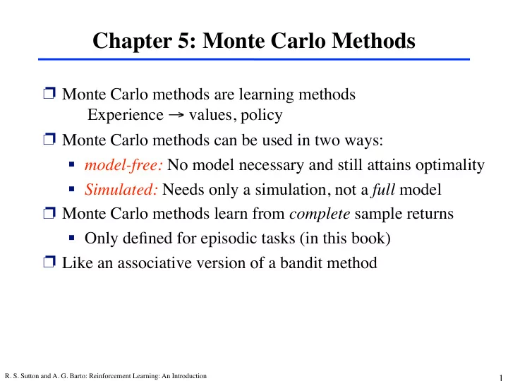
Chapter 5: Monte Carlo Methods ❐ Monte Carlo methods are learning methods 
 Experience → values, policy ❐ Monte Carlo methods can be used in two ways: ! model-free: No model necessary and still attains optimality ! Simulated: Needs only a simulation, not a full model ❐ Monte Carlo methods learn from complete sample returns ! Only defined for episodic tasks (in this book) ❐ Like an associative version of a bandit method R. S. Sutton and A. G. Barto: Reinforcement Learning: An Introduction 1

Monte Carlo Policy Evaluation ❐ Goal: learn v π ( s ) ❐ Given: some number of episodes under π which contain s ❐ Idea: Average returns observed after visits to s 5 1 2 3 4 ❐ Every-Visit MC: average returns for every time s is visited in an episode ❐ First-visit MC: average returns only for first time s is visited in an episode ❐ Both converge asymptotically R. S. Sutton and A. G. Barto: Reinforcement Learning: An Introduction 2

First-visit Monte Carlo policy evaluation Initialize: π ← policy to be evaluated V ← an arbitrary state-value function Returns ( s ) ← an empty list, for all s ∈ S Repeat forever: Generate an episode using π For each state s appearing in the episode: G ← return following the first occurrence of s Append G to Returns ( s ) V ( s ) ← average( Returns ( s )) R. S. Sutton and A. G. Barto: Reinforcement Learning: An Introduction 3

Blackjack example ❐ Object: Have your card sum be greater than the dealer’s without exceeding 21. ❐ States (200 of them): ! current sum (12-21) ! dealer’s showing card (ace-10) ! do I have a useable ace? ❐ Reward: +1 for winning, 0 for a draw, -1 for losing ❐ Actions: stick (stop receiving cards), hit (receive another card) ❐ Policy: Stick if my sum is 20 or 21, else hit ❐ No discounting ( 휸 = 1) R. S. Sutton and A. G. Barto: Reinforcement Learning: An Introduction 4

Learned blackjack state-value functions R. S. Sutton and A. G. Barto: Reinforcement Learning: An Introduction 5

Backup diagram for Monte Carlo ❐ Entire rest of episode included ❐ Only one choice considered at each state (unlike DP) ! thus, there will be an explore/exploit dilemma ❐ Does not bootstrap from successor states’s values (unlike DP) ❐ Time required to estimate one state does not depend on the terminal state total number of states R. S. Sutton and A. G. Barto: Reinforcement Learning: An Introduction 6

The Power of Monte Carlo e.g., Elastic Membrane (Dirichlet Problem) How do we compute the shape of the membrane or bubble? R. S. Sutton and A. G. Barto: Reinforcement Learning: An Introduction 7

Two Approaches Relaxation Kakutani’s algorithm, 1945 R. S. Sutton and A. G. Barto: Reinforcement Learning: An Introduction 8

Monte Carlo Estimation of Action Values (Q) ❐ Monte Carlo is most useful when a model is not available ! We want to learn q * ❐ q π ( s,a ) - average return starting from state s and action a following π ❐ Converges asymptotically if every state-action pair is visited ❐ Exploring starts: Every state-action pair has a non-zero probability of being the starting pair R. S. Sutton and A. G. Barto: Reinforcement Learning: An Introduction 9

Monte Carlo Control evaluation Q q π Q π π greedy( Q ) improvement ❐ MC policy iteration: Policy evaluation using MC methods followed by policy improvement ❐ Policy improvement step: greedify with respect to value (or action-value) function R. S. Sutton and A. G. Barto: Reinforcement Learning: An Introduction 10

Convergence of MC Control ❐ Greedified policy meets the conditions for policy improvement: q π k ( s, π k +1 ( s )) = q π k ( s, argmax q π k ( s, a )) a = max q π k ( s, a ) a q π k ( s, π k ( s )) ≥ ≥ = v π k ( s ) . ❐ And thus must be ≥ π k by the policy improvement theorem ❐ This assumes exploring starts and infinite number of episodes for MC policy evaluation ❐ To solve the latter: ! update only to a given level of performance ! alternate between evaluation and improvement per episode R. S. Sutton and A. G. Barto: Reinforcement Learning: An Introduction 11

Monte Carlo Exploring Starts Initialize, for all s ∈ S , a ∈ A ( s ): Fixed point is optimal Q ( s, a ) ← arbitrary policy π * π ( s ) ← arbitrary Returns ( s, a ) ← empty list Now proven (almost) Repeat forever: Choose S 0 ∈ S and A 0 ∈ A ( S 0 ) s.t. all pairs have probability > 0 Generate an episode starting from S 0 , A 0 , following π For each pair s, a appearing in the episode: G ← return following the first occurrence of s, a Append G to Returns ( s, a ) Q ( s, a ) ← average( Returns ( s, a )) For each s in the episode: π ( s ) ← argmax a Q ( s, a ) R. S. Sutton and A. G. Barto: Reinforcement Learning: An Introduction 12

Blackjack example continued ❐ Exploring starts ❐ Initial policy as described before ! * V * v * * * 1 0 21 STICK 20 19 21 21 Usable 18 + 1 17 ace 16 Player sum " 1 15 A A HIT 14 13 Dealer showing 12 11 A 2 3 4 5 6 7 8 9 10 12 12 1 1 0 0 21 20 Player sum 19 STICK 21 No 18 21 + 1 17 usable 16 Player sum Player sum " 1 15 ace A A 14 HIT 13 Dealer showing D e 12 a l e r 11 s h o A 2 3 4 5 6 7 8 9 10 w i n 12 g 12 Dealer showing 1 1 0 0 R. S. Sutton and A. G. Barto: Reinforcement Learning: An Introduction 13

On-policy Monte Carlo Control ❐ On-policy: learn about policy currently executing ❐ How do we get rid of exploring starts? ! The policy must be eternally soft : – π ( a | s ) > 0 for all s and a ! e.g. ε -soft policy: ✏ ✏ – probability of an action = or ) + 1 − ✏ + | A ( s ) | | A ( s ) | h max (greedy) non-max ❐ Similar to GPI: move policy towards greedy policy 
 (e.g., ε -greedy) ❐ Converges to best ε -soft policy R. S. Sutton and A. G. Barto: Reinforcement Learning: An Introduction 14

On-policy MC Control Initialize, for all s 2 S , a 2 A ( s ): Q ( s, a ) arbitrary Returns ( s, a ) empty list ⇡ ( a | s ) an arbitrary " -soft policy Repeat forever: (a) Generate an episode using ⇡ (b) For each pair s, a appearing in the episode: G return following the first occurrence of s, a Append G to Returns ( s, a ) Q ( s, a ) average( Returns ( s, a )) (c) For each s in the episode: A ∗ arg max a Q ( s, a ) For all a 2 A ( s ): ⇢ 1 � " + " / | A ( s ) | if a = A ∗ ⇡ ( a | s ) " / | A ( s ) | if a 6 = A ∗ R. S. Sutton and A. G. Barto: Reinforcement Learning: An Introduction 15

What we’ve learned about Monte Carlo so far ❐ MC has several advantages over DP: ! Can learn directly from interaction with environment ! No need for full models ! No need to learn about ALL states (no bootstrapping) ! Less harmed by violating Markov property (later in book) ❐ MC methods provide an alternate policy evaluation process ❐ One issue to watch for: maintaining sufficient exploration ! exploring starts, soft policies R. S. Sutton and A. G. Barto: Reinforcement Learning: An Introduction 22

Off-policy methods ❐ Learn the value of the target policy π from experience due to behavior policy 휇 ❐ For example, π is the greedy policy (and ultimately the optimal policy) while 휇 is exploratory (e.g., 휀 -soft) ❐ In general, we only require coverage , i.e., that 휇 generates behavior that covers, or includes, π es µ ( a | s ) > 0. for every s,a at which at π ( a | s ) > 0 ❐ Idea: importance sampling – Weight each return by the ratio of the probabilities of the trajectory under the two policies 17

Importance Sampling Ratio ❐ Probability of the rest of the trajectory, after S t , under π : Pr { A t , S t +1 , A t +1 , . . . , S T | S t , A t : T − 1 ∼ π } = π ( A t | S t ) p ( S t +1 | S t , A t ) π ( A t +1 | S t +1 ) · · · p ( S T | S T − 1 , A T − 1 ) T − 1 Y = π ( A k | S k ) p ( S k +1 | S k , A k ) , k = t ❐ In importance sampling, each return is weighted by the relative probability of the trajectory under the two policies T − 1 Q T − 1 k = t π ( A k | S k ) p ( S k +1 | S k , A k ) π ( A k | S k ) ρ T Y t = = µ ( A k | S k ) . Q T − 1 k = t µ ( A k | S k ) p ( S k +1 | S k , A k ) k = t ❐ This is called the importance sampling ratio ❐ All importance sampling ratios have expected value 1  π ( A k | S k ) � µ ( a | S k ) π ( a | S k ) X X = µ ( a | S k ) = π ( a | S k ) = 1 . E A k ∼ µ µ ( A k | S k ) a a 18

Importance Sampling ❐ New notation: time steps increase across episode boundaries: ! . . . s . . . . ▨ . . . . . . ▨ . . . s . . . . ▨ . . . ! t = 1 2 3 4 5 6 7 8 9 10 11 12 13 14 15 16 17 18 19 20 21 22 23 24 25 26 27 T ( s ) = { 4 , 20 } T (4) = 9 T (20) = 25 set of start times next termination times ❐ Ordinary importance sampling forms estimate t ∈ T ( s ) ρ T ( t ) P G t V ( s ) . t = . | T ( s ) | ❐ Whereas weighted importance sampling forms estimate t ∈ T ( s ) ρ T ( t ) P G t V ( s ) . t = t ∈ T ( s ) ρ T ( t ) P t 19