Sequential Importance Sampling for Rare Event Estimation with - PowerPoint PPT Presentation
Sequential Importance Sampling for Rare Event Estimation with Computer Experiments Brian Williams and Rick Picard LA-UR-12-22467 Statistical Sciences Group, Los Alamos National Laboratory Abstract Importance sampling often drastically
Sequential Importance Sampling for Rare Event Estimation with Computer Experiments Brian Williams and Rick Picard LA-UR-12-22467 Statistical Sciences Group, Los Alamos National Laboratory
Abstract Importance sampling often drastically improves the variance of percentile and quantile estimators of rare events. We propose a sequential strategy for iterative refinement of importance distributions for sampling uncertain inputs to a computer model to estimate quantiles of model output or the probability that the model output exceeds a fixed or random threshold. A framework is introduced for updating a model surrogate to maximize its predictive capability for rare event estimation with sequential importance sampling. Examples of the proposed methodology involving materials strength and nuclear reactor applications will be presented. Slide 1
Outline • Interested in rare event estimation – Outputs obtained from computational model – Uncertainties in operating conditions and physics variables – Physics variables calibrated wrt reference experimental data • In particular, quantile or percentile estimation – One of q α or α is specified and the other is to be inferred – q α may be random when inferring α • Sequential importance sampling for improved inference – Oversample region of parameter space producing rare events of interest – Sequentially refine importance distributions for improved inference Slide 2
Examples • Risk of released airborne load colliding with aircraft – For control variable settings of interest, inference on probability of danger • Structural reliability benchmark – Inference on probability of failure of a four-branch series system • Catastrophe due to pyroclastic flows – Inference on probability of catastrophe within t years • Volume of storage in sewer system required to meet certain environmental standards – Inference on 95 th quantile • Pressurizer failure in nuclear reactor loop – Inference on probability of dangerous peak coolant temperature Slide 3
Percentile Estimates • q α fixed PDF of operating PDF of physics conditions variables – Monte Carlo estimate of α and associated uncertainty obtained via samples {( x (j) , θ (j) ), j=1,…,N} from the product density f( x ) π ( θ ) • Random threshold q α having PDF h( q ) and CDF H( q ) – Brute force – Improvement via Rao-Blackwellization Slide 4
Quantile Estimates • Percentile α fixed • Obtain samples {( x (j) , θ (j) ), j=1,…,N} from the product density f( x ) π ( θ ) • Evaluate computational model on samples, { η ( x (j) , θ (j) ), j=1,…,N} • Sort code evaluations and choose an appropriate order statistic from the list – e.g. if α = 0.001 and N=10,000, choose the 11-th largest value – Quantile estimates from simulations are not unique, e.g. any value between the 10-th and 11-th largest values may be chosen • Uncertainty obtained e.g. by inverting binomial confidence intervals Slide 5
Importance Sampling • Sample from alternative distribution g( x , θ ), evaluate computational model, and weight each output Importance weight Importance density – percentile estimator: – quantile estimator: Smallest value of q α for which • Importance density g( x , θ ) ideally chosen to increase the likelihood of observing desired rare events – Such knowledge may initially be vague: how to proceed? minimum variance importance density Slide 6
Relevant (Sensitive) Variables • A subset of variables may be responsible for generating rare events – Relevant x r , θ r – Irrelevant x i , θ i • Minimum variance importance distribution • Importance distribution g( x , θ ) becomes Slide 7
Example: PTW Material Strength Model strain rate activation energy yield stress T/ T m ( ρ ) saturation stress T = temperature atomic vibration time T m ( ρ ) = melting temp. strain stress Model parameters θ θ Calibrated to experimental data Multivariate Normal Input conditions x Independent normal distributions Slide 8
Adaptive Importance Sampling • Choose g( x , θ ) by iterative refinement 1. Sample from initial importance density g (1) ( x , θ ) = f( x ) π ( θ ) 2. Given target probability or quantile level, determine which parameters are sensitive for producing large output values e.g. for target 0.0001 quantile, examine the 100 largest output order statistics – calculated from 10 6 samples and compare the corresponding parameter samples to random parameter samples 1-in-10,000 Random 1-in-100,000 Slide 9
Adaptive Importance Sampling 3. For sensitive parameters in (2), adopt a family of importance densities (e.g. Beta, (truncated) Normal, etc.). Fit the parameters of this family to the selected largest order statistics (e.g. method of moments, MLE). 4. Keep the conditional distribution from (1) for the insensitive parameters, given values of the sensitive parameters. 5. Combine the distributions of (3) and (4) to obtain g (2) ( x , θ ). 6. Repeat (2)-(5) until the updated importance distribution g (k) ( x , θ ) “stabilizes” in its approximation of the minimum variance importance distribution. Means, variances, and covariances of sensitive parameters are now estimated via their conditional distributions based on a random sample from g (k) ( x , θ ), e.g. Slide 10
Results: Variance Reduction • Four sensitive PTW variables: • Define variance reduction factor: VRF = Brute Force Variance Variance of IS quantity VRF > 1 : Importance Sampling Favored Target Quantile: 0.0001 0.001 0.0001 0.00001 0.000001 4-D VRF 3 3231 2245 225 10-D VRF 0.3 1237 204 20 Slide 11
Results: Adaptive Importance Sampling • Four sensitive PTW variables: • Results of iterative process: Minimum Variance Convergence often achieved rapidly! Importance Dist’n Slide 12
Normalized Importance Sampling Estimates • In many applications, π ( θ ) is a posterior distribution with unknown normalizing constant: π ( θ ) = c norm k( θ ) • Modified weights and estimators: – Although , w distribution has a sample mean (SD) of 0.007 (4.1) based on 10 6 samples – 98% of weights less than sample mean Target Quantile: 0.0001 0.001 0.0001 0.00001 0.000001 4-D q 1512.6 1566.0 1610.5 1649.0 10-D q 1509.9 1566.0 1610.4 1648.7 Normalized q 1615.7 1653.8 1679.0 1718.8 Slide 13
Many Applications Will Require Code Surrogates • Many computational models run too slowly for direct use in brute force or importance sampling based rare event inference • Use training runs to develop a statistical surrogate model for the complex code (i.e., the emulator ) based on a Gaussian process – Deterministic code is interpolated with zero uncertainty outputs evaluated at training runs z 1 ,..., z n • Kriging Predict correlations between pairwise correlations prediction site z and between training training runs z 1 ,..., z n runs z 1 ,..., z n • Kriging Variance Slide 14
Previous Work • Oakley, J. (2004). “Estimating percentiles of uncertain computer code outputs,” Applied Statistics , 53, 83-93. • Quantile estimation with α = 0.05 • Assuming a Gaussian Process model for unsampled code output: – Generate a random function η (i) (.) from the posterior process – Use Monte Carlo methods to estimate q 0.05,(i) – Repeat previous steps to obtain a sample q 0.05,(1) ,…, q 0.05,(K) • Sequential design to improve emulation in relevant region of input space – First stage: space-filling to learn about η (.) globally – Second stage: IMSE criterion with weight function chosen as a density estimate from the K inputs corresponding to q 0.05,(1) ,…, q 0.05,(K) Slide 15
Surrogate-based Percentile/Quantile Estimation • Gaussian Process model with plug-in covariance parameter estimates, e.g. • Process-based inference Slide 16
Surrogate Bias May Affect Inference Results • Example: Approximation of PTW model based on 55 runs – Importance distributions and efficiencies based on surrogate are similar to those based on direct model calls … Mean Standard Deviation T p s 0 T p s 0 True 82 2.27 1.66 0.0105 21 2.1 0.18 0.00045 Surr. 95 4.25 1.73 0.0104 23 1.6 0.17 0.00047 – However, quantile estimates from surrogate can be “significantly” different than the “true values” relative to Monte Carlo Uncertainty 1566.0 (true) vs. 1549.3 (surrogate) for target quantile of 0.0001 Slide 17
Convergence Assessment Through Iterative Refinement of Surrogate • Choose design augmentation that minimizes integrated mean square error with respect to the currently estimated importance distributions for sensitive parameters – A version of “targeted” IMSE (tIMSE) Estimate correlation parameters For sensitive input i , select w i ( z i ) based on current design D 0 to be its importance distribution Slide 18
Uncorrelated Importance Sampling • Importance distribution g (k) ( x , θ ) is multivariate Gaussian • IMSE calculation: Obtaining uncorrelated variables – Relevant (sensitive) quantities – Insensitive quantities – Transformations – Similar for insensitive variables Slide 19
Quantile Estimates May Converge Quickly… Target quantile 0.0001 Quantile bias at convergence consistent with “average” single-stage design surrogate error Surrogate quality +5; +10 in importance region may benefit from higher frequency updates Slide 20
Recommend
More recommend
Explore More Topics
Stay informed with curated content and fresh updates.
