Section 18.7 Artificial Neural Networks CS4811 - Artificial - PowerPoint PPT Presentation
Section 18.7 Artificial Neural Networks CS4811 - Artificial Intelligence Nilufer Onder Department of Computer Science Michigan Technological University Outline Brains Regression problems Neural network structures Single-layer perceptrons
Section 18.7 Artificial Neural Networks CS4811 - Artificial Intelligence Nilufer Onder Department of Computer Science Michigan Technological University
Outline Brains Regression problems Neural network structures Single-layer perceptrons Multilayer perceptrons (MLPs) Back-propagation learning Applications of neural networks
Brains ◮ 10 11 neurons of > 20 types, 1ms-10ms cycle time ◮ Signals are noisy “spike trains” of electrical potential
Linear regression ◮ The graph in (a) shows the data points of price ( y ) versus floor space ( x ) of houses for sale in Berkeley, CA, in July 2009. ◮ The dotted line is a linear function hypothesis that minimizes squared error: y = 0 . 232 x + 246 ◮ The graph in (b) is the plot of the loss function j ( w 1 x j + w 0 − y j ) 2 for various values of w 0 and w 1 . � ◮ Note that the loss function is convex, with a single global mimimum.
Linear classifiers with a hard threshold ◮ The plots show two seismic data parameters, body wave magnitude x 1 and surface wave magnitute x 2 . ◮ Nuclear explosions are shown as black circles. Earthquakes (not nuclear explosions) are shown as white circles. ◮ In graph (a), the line separates the positive and negative examples.
McCulloch-Pitts “unit” ◮ Output is a “squashed” linear function of the inputs �� � a i ← g ( in i ) = g j W j , i a j ◮ It is a gross oversimplification of real neurons, but its purpose is to develop an understanding of what networks of simple units can do
Activation functions ◮ (a) is a step function or threshold function ◮ (b) is a sigmoid function 1 / (1 + e − x ) ◮ Changing the bias weight W 0 , i moves the threshold location
Implementing logical functions McCulloch and Pitts: every Boolean function can be implemented
Neural Network structures ◮ Feed-forward networks: implement functions, no internal state ◮ single-layer perceptrons ◮ multi-layer perceptrons ◮ Recurrent networks: have directed cycles with delays, have internal state, can oscillate ◮ (Hopfield networks) ◮ (Boltzmann machines)
Feed-forward example ◮ Feed-forward network: parameterized family of nonlinear functions ◮ Output of unit 5 is a 5 = g ( W 3 , 5 · a 3 + W 4 , 5 · a 4 ) = g ( W 3 , 5 · g ( W 1 , 3 · a 1 + W 2 , 3 · a 2 )+ W 4 , 5 · g ( W 1 , 4 · a 1 + W 2 , 4 · a 2 )) ◮ Adjusting the weights changes the function: do learning this way!
Single-layer perceptrons ◮ Output units all operate separately – no shared weights ◮ Adjusting the weights moves the location, orientation, and steepness of cliff
Expressiveness of perceptrons ◮ Consider a perceptron where g is the step function (Rosenblatt, 1957, 1960) ◮ It can represent AND, OR, NOT, but not XOR ◮ Minsky & Papert (1969) pricked the neural network balloon ◮ A perceptron represents a linear separator in input space: � j W j x j > 0 or W · x > 0
Perceptron learning ◮ Learn by adjusting weights to reduce error on training set ◮ The squared error for an example with input x and true output y is 2 Err 2 ≡ 1 E = 1 2 ( y − h W ( x )) 2
Perceptron learning (cont’d) ◮ Perform optimization search by gradient descent: n ∂ E Err × ∂ Err ∂ � = = Err × y − g ( W j x j ) ∂ W j ∂ W j ∂ W j j =0 − Err × g ′ ( in ) × x j = ◮ Simple weight update rule: W j ← W j + ( α × g ′ ( in )) × Err × x j ◮ Err = y − h W = 1 − 1 = 0 ⇒ no change ◮ Err = y − h W = 1 − 0 = 1 ⇒ increase w i when x i is positive, decrease otherwise ◮ Err = y − h W = 0 − 1 = − 1 ⇒ decrease w i when x i is positive, decrease otherwise ◮ Perceptron learning rule converges to a consistent function for any linearly separable data set
Multilayer perceptrons (MLPs) ◮ Layers are usually fully connected ◮ Numbers of hidden units are typically chosen by hand
Expressiveness of MLPs ◮ All continuous functions with 2 layers, all functions with 3 layers ◮ Ridge: Combine two opposite-facing threshold functions ◮ Bump: Combine two perpendicular ridges ◮ Add bumps of various sizes and locations to fit any surface ◮ Proof requires exponentially many hidden units
Back-propagation learning Output layer: same as for single-layer perceptron, W j , i ← W j , i + α × a j × ∆ i where ∆ i = Err i × g ′ ( in i ) Hidden layer: back-propagate the error from the output layer: ∆ j = g ′ ( in j ) � i w j , i ∆ i . Update rule for weights in hidden layer: W k , j ← W k , j + α × a k × ∆ j . (Most neuroscientists deny that back-propagation occurs in the brain)
Back-propagation derivation The squared error on a single example is defined as E = 1 ( y i − a i ) 2 , � 2 i where the sum is over the nodes in the output layer. ∂ E − ( y i − a i ) ∂ a i = − ( y i − a i ) ∂ g ( in i ) = ∂ W j , i ∂ W j , i ∂ W j , i − ( y i − a i ) g ′ ( in i ) ∂ in i = ∂ W ji ∂ � = − ( y i − a i ) g ′ ( in i ) W j , i a j ∂ W j , i j − ( y i − a i ) g ′ ( in i ) a j = − a j ∆ i =
Back-propagation derivation (cont’d) ∂ E ( y i − a i ) ∂ a i ( y i − a i ) ∂ g ( in i ) � � = = − − ∂ W k , j ∂ W k , j ∂ W k , j i i ( y i − a i ) g ′ ( in i ) ∂ in i ∂ � � � = = − ∆ i W y , i a j − ∂ W k , j ∂ W k , j i i j ∂ a j ∂ g ( in j ) � � = ∆ i W y , i = − ∆ i W y , i − ∂ W k , j ∂ W k , j i i ∆ i W y , i g ′ Jin j ) ∂ in j � = − ∂ W k , j i �� � ∂ � ∆ i W y , i g ′ ( in j ) = W k , j a k − ∂ W k , j i k � ∆ i W y , i g ′ ( in j ) a k = − a k ∆ j = − i
MLP learners ◮ MLPs are quite good for complex pattern recognition tasks ◮ The resulting hypotheses cannot be understood easily ◮ Typical problems: slow convergence, local minima
Handwritten digit recognition ◮ 3-nearest-neighbor classifier (stored images) = 2.4% error ◮ Shape matching based on computer vision = 0.63% error ◮ 400-300-10 unit MLP = 1.6% error ◮ LeNet 768-192-30-10 unit MLP = 0.9% error ◮ Boosted neural network = 0.7% error ◮ Support vector machine = 1.1% error ◮ Current best: virtual support vector machine = 0.56% error ◮ Humans ≈ 0.2% error
Summary ◮ Brains have lots of neurons; each neuron ≈ linear–threshold unit (?) ◮ Perceptrons (one-layer networks) are insufficiently expressive ◮ Multi-layer networks are sufficiently expressive; can be trained by gradient descent, i.e., error back-propagation ◮ Many applications: speech, driving, handwriting, fraud detection, etc. ◮ Engineering, cognitive modelling, and neural system modelling subfields have largely diverged
Sources for the slides ◮ AIMA textbook (3 rd edition) ◮ AIMA slides: http://aima.cs.berkeley.edu/ ◮ Neuron cell: http://www.enchantedlearning.com/subjects/anatomy/brain/Neuron.shtml (Accessed December 10, 2011)
Recommend
More recommend
Explore More Topics
Stay informed with curated content and fresh updates.
