Search in High-Dimensional spaces and Dimensionality Reduction i - PDF document

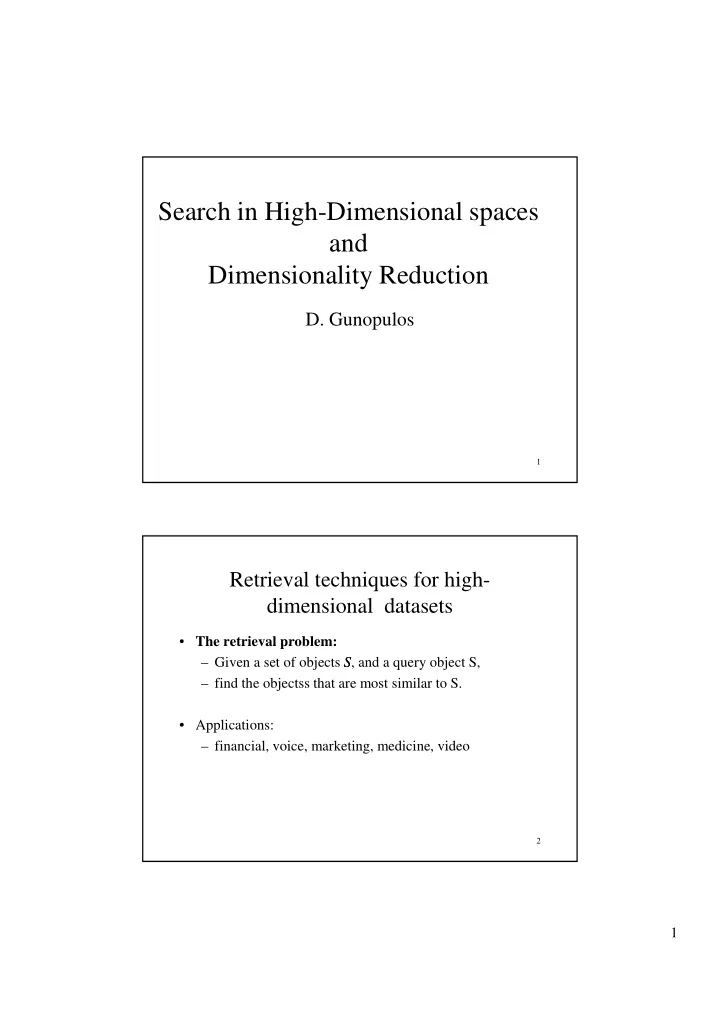
Search in High-Dimensional spaces and Dimensionality Reduction i i li d i D. Gunopulos 1 Retrieval techniques for high- dimensional datasets • The retrieval problem: The retrieval problem: – Given a set of objects S , and a query object S, – find the objectss that are most similar to S. • Applications: – financial, voice, marketing, medicine, video g 2 1

Examples • Find companies with similar stock prices over a time Find companies with similar stock prices over a time interval • Find products with similar sell cycles • Cluster users with similar credit card utilization • Cluster products 3 Indexing when the triangle inequality holds • Typical distance metric: L norm Typical distance metric: L p norm. • We use L 2 as an example throughout: – D(S,T) = ( Σ i=1,..,n (S[i] - T[i]) 2 ) 1/2 4 2

Indexing: The naïve way • Each object is an n-dimensional tuple Each object is an n dimensional tuple • Use a high-dimensional index structure to index the tuples • Such index structures include – R-trees, – kd-trees, – vp-trees, p – grid-files... 5 High-dimensional index structures • All require the triangle inequality to hold All require the triangle inequality to hold • All partition either – the space or – the dataset into regions • The objective is to: – search only those regions that could potentially contain y g p y good matches – avoid everything else 6 3

The naïve approach: Problems • High-dimensionality: High dimensionality: – decreases index structure performance (the curse of dimensionality) – slows down the distance computation • Inefficiency 7 Dimensionality reduction • The main idea: reduce the dimensionality of the space The main idea: reduce the dimensionality of the space. • Project the n-dimensional tuples that represent the time series in a k-dimensional space so that: – k << n – distances are preserved as well as possible 8 4

Dimensionality Reduction • Use an indexing technique on the new space Use an indexing technique on the new space. • GEMINI ([Faloutsos et al]): – Map the query S to the new space – Find nearest neighbors to S in the new space – Compute the actual distances and keep the closest 9 Dimensionality Reduction • A time series is represented as a k dim point • A time series is represented as a k-dim point • The query is also transformed to the k-dim space query f2 dataset f1 time 10 5

Dimensionality Reduction • Let F be the dimensionality reduction technique: Let F be the dimensionality reduction technique: – Optimally we want: – D(F(S), F(T) ) = D(S,T) • Clearly not always possible. • If D(F(S), F(T) ) ≠ D(S,T) – false dismissal (when D(S,T) << D(F(S), F(T) ) ) ( ( ) ( ( ) ( ) ) ) – false positives (when D(S,T) >> D(F(S), F(T) ) ) 11 Dimensionality Reduction • To guarantee no false dismissals we must be able to prove To guarantee no false dismissals we must be able to prove that: – D(F(S),F(T)) < a D(S,T) – for some constant a • a small rate of false positives is desirable, but not essential 12 6

What we achieve • Indexing structures work much better in lower Indexing structures work much better in lower dimensionality spaces • The distance computations run faster • The size of the dataset is reduced, improving performance. 13 Dimensionality Techniques • We will review a number of dimensionality techniques that We will review a number of dimensionality techniques that can be applied in this context – SVD decomposition, – Discrete Fourier transform, and Discrete Cosine transform – Wavelets – Partitioning in the time domain – Random Projections j – Multidimensional scaling – FastMap and its variants 14 7

SVD decomposition - the Karhunen- Loeve transform • Intuition: find the axis that Intuition: find the axis that shows the greatest variation, and project all points into this axis • [Faloutsos, 1996] 15 SVD: The mathematical formulation • Find the eigenvectors of Find the eigenvectors of the covariance matrix • These define the new space • The eigenvalues sort them in “goodness” order order 16 8

SVD: The mathematical formulation, Cont’d • Let A be the M x n matrix of M time series of length n Let A be the M x n matrix of M time series of length n • The SVD decomposition of A is: = U x L x V T , – U, V orthogonal – L diagonal • L contains the eigenvalues of A T A M x n n x n n x n V U x L x 17 SVD Cont’d • To approximate the time To approximate the time X series, we use only the k X' largest eigenvectors of C. 0 20 40 60 80 100 120 140 • A’ = U x L k eigenwave 0 eigenwave 1 • A’ is an M x k matrix eigenwave 2 eigenwave 3 eigenwave 4 eigenwave 5 eigenwave 6 eigenwave 7 18 9

SVD Cont’d • Advantages: Advantages: – Optimal dimensionality reduction (for linear projections) • Disadvantages: – Computationally hard, especially if the time series are very long. – Does not work for subsequence indexing 19 SVD Extensions • On-line approximation algorithm On line approximation algorithm – [Ravi Kanth et al, 1998] • Local diemensionality reduction: – Cluster the time series, solve for each cluster – [Chakrabarti and Mehrotra, 2000], [Thomasian et al] 20 10

Discrete Fourier Transform • Analyze the frequency spectrum of an one dimensional Analyze the frequency spectrum of an one dimensional signal • For S = (S 0 , …,S n-1 ), the DFT is: • S f = 1/ √ n Σ i=0,..,n-1 S i e -j2 π fi/n f = 0,1,…n-1, j 2 =-1 • An efficient O(nlogn) algorithm makes DFT a practical method • [Agrawal et al, 1993], [Rafiei and Mendelzon, 1998] 21 Discrete Fourier Transform • To approximate the time To approximate the time X series, keep the k largest X' Fourier coefficients only. 0 20 40 60 80 100 120 140 • Parseval’s theorem: Σ i=0,..,n-1 S i 2 = Σ i=0,..,n-1 S f 0 2 1 • DFT is a linear transform so: 2 3 – Σ i=0,..,n-1 (S i -T i ) 2 = Σ i=0,..,n-1 (S f -T f ) 2 22 11

Discrete Fourier Transform • Keeping k DFT coefficients lower bounds the distance: Keeping k DFT coefficients lower bounds the distance: – Σ i=0,..,n-1 (S[i]-T[i]) 2 > Σ i=0,..,k-1 (S f -T f ) 2 • Which coefficients to keep: – The first k (F-index, [Agrawal et al, 1993], [Rafiei and Mendelzon, 1998]) Mendelzon, 1998]) – Find the optimal set (not dynamic) [R. Kanth et al, 1998] 23 Discrete Fourier Transform • Advantages: Advantages: – Efficient, concentrates the energy • Disadvantages: – To project the n-dimensional time series into a k- dimensional space, the same k Fourier coefficients must be store for all series – This is not optimal for all series – To find the k optimal coefficients for M time series, compute the average energy for each coefficient 24 12

Wavelets • Represent the time series as a sum of prototype functions Represent the time series as a sum of prototype functions like DFT • Typical base used: Haar wavelets • Difference from DFT: localization in time • Can be extended to 2 dimensions • [Chan and Fu, 1999] • Has been very useful in graphics, approximation techniques 25 Wavelets • An example (using the Haar wavelet basis) An example (using the Haar wavelet basis) – S ≡ (2, 2, 7, 9) : original time series – S’ ≡ (5, 6, 0, 2) : wavelet decomp. – S[0] = S’[0] - S’[1]/2 - S’[2]/2 – S[1] = S’[0] - S’[1]/2 + S’[2]/2 – S[2] = S’[0] + S’[1]/2 - S’[3]/2 [ ] [ ] [ ] [ ] – S[3] = S’[0] + S’[1]/2 + S’[3]/2 • Efficient O(n) algorithm to find the coefficients 26 13

Using wavelets for approximation • Keep only k coefficients Keep only k coefficients, X approximate the rest with 0 X' • Keeping the first k coefficients: – equivalent to low pass filtering 0 20 40 60 80 100 120 140 Haar 0 • Keeping the largest k coefficients: Haar 1 Haar 2 – More accurate representation, Haar 3 Haar 4 Haar 5 But not useful for indexing Haar 6 Haar 7 27 Wavelets • Advantages: Advantages: – The transformed time series remains in the same (temporal) domain – Efficient O(n) algorithm to compute the transformation • Disadvantages: – Same with DFT 28 14

Line segment approximations • Piece-wise Aggregate Approximation Piece wise Aggregate Approximation – Partition each time series into k subsequences (the same for all series) – Approximate each sequence by : • its mean and/or variance: [Keogh and Pazzani, 1999], [Yi and Faloutsos, 2000] • a line segment: [Keogh and Pazzani, 1998] 29 Temporal Partitioning • Very Efficient technique Very Efficient technique (O(n) time algorithm) X X' • Can be extended to address the subsequence matching 0 20 40 60 80 100 120 140 problem x 0 x 1 • Equivalent to wavelets (when x 2 x 3 k= 2 i and mean is used) k= 2 , and mean is used) x 4 x 4 x 5 x 6 x 7 30 15