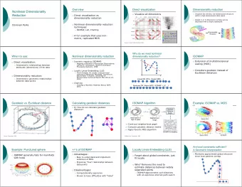
Visualization ( Nonlinear dimensionality reduction ) Fei Sha - PowerPoint PPT Presentation

Visualization ( Nonlinear dimensionality reduction ) Fei Sha Yahoo! Research feisha@yahoo-inc.com CS294 March 18, 2008

Dimensionality reduction • Question: How can we detect low dimensional structure in high dimensional data? • Motivations: Exploratory data analysis & visualization Compact representation Robust statistical modeling

Linear dimensionality reductions • Many examples (Percy’s lecture on 2/19/2008) Principal component analysis (PCA) Fischer discriminant analysis (FDA) Nonnegative matrix factorization (NMF) • Framework x ∈ ℜ D → y ∈ ℜ d D ≫ d y = Ux linear transformation of original space

Linear methods are not sufficient • What if data is “nonlinear”? !# classic toy !" # example of " Swiss roll ! # ! !" ! !# %" $" !# !" !" # " ! # " ! !" $# • PCA results !" !# " # ! " ! !# ! !" ! !" ! !# ! " # " !# !"

What we really want is “unrolling” !#$ !# ! !" "#$ " # %#$ nonlinear " % ! # mapping ! %#$ ! !" ! " ! "#$ ! !# %" ! ! $" !# !" !" # " ! !#$ ! # " ! !" ! ! ! "#$ ! " ! %#$ % %#$ " "#$ ! !#$ Simple geometric intuition: distortion in local areas faithful in global structure

Outline • Linear method: redux and new intuition Multidimensional scaling (MDS) • Graph based spectral methods Isomap Locally linear embedding • Other nonlinear methods Kernel PCA Maximum variance unfolding (MVU)

Linear methods: redux PCA: does the data mostly lie in a subspace? If so, what is its dimensionality? D = 2 D = 3 d = 1 d = 2

The framework of PCA • Assumption: � x i = 0 Centered inputs i Projection into subspace y i = Ux i UU T = I (note: a small change from • Interpretation Percy’s notation) maximum variance preservation � � y i � 2 arg max i minimum reconstruction errors � � x i − U T y i � 2 arg min i

Other criteria we can think of... How about preserve pairwise distances? � x i − x j � = � y i − y j � This leads to a new type of linear methods multidimensional scaling (MDS) Key observation: from distances to inner products � x i − x j � 2 = x T i x i − 2 x T i x j + x T j x j

Recipe for multidimensional scaling • Compute Gram matrix on centered points G = X T X X = ( x 1 , x 2 , . . . , x N ) • Diagonalize � λ 1 ≥ λ 2 ≥ · · · ≥ λ N λ i v i v T G = i • Derive outputs and estimate dimensionality i � d � � d = min arg max 1 λ i ≥ THRESHOLD i =1 � λ i v id y id =

MDS when only distances are known We convert distance matrix D = { d 2 d 2 ij = � x i − x j � 2 ij } to Gram matrix G = − 1 2 HDH with centering matrix H = I n − 1 n 11 T

PCA vs MDS: is MDS really that new? • Same set of eigenvalues N XX T v = λ v → X T X 1 1 N X T v = N λ 1 N X T v PCA diagonalization MDS diagonalization • Similar low dimensional representation • Different computational cost PCA scales quadratically in D MDS scales quadratically in N Big win for MDS when D is much greater than N !

How to generalize to nonlinear structures? All we need is a simple twist on MDS

5min Break?

Nonlinear structures • Manifolds such as • can be approximately locally with linear structures. This is a key intuition that we will repeatedly appeal to

Manifold learning Given high dimensional data sampled from a low dimensional nonlinear submanifold, how to compute a faithful embedding? Input Output { y i ∈ ℜ d , i = 1 , 2 , . . . , n } { x i ∈ ℜ D , i = 1 , 2 , . . . , n }

Outline • Linear method: redux and new intuition Multidimensional scaling (MDS) • Graph based spectral methods Isomap Locally linear embedding • Other nonlinear methods Kernel PCA Maximum variance unfolding

A small jump from MDS to Isomap • Key idea MDS Preserve pairwise Euclidean distances • Algorithm in a nutshell Estimate geodesic distance along submanifold Perform MDS as if the distances are Euclidean

A small jump from MDS to Isomap • Key idea Isomap Preserve pairwise geodesic distances • Algorithm in a nutshell Estimate geodesic distance along submanifold Perform MDS as if the distances are Euclidean

Why geodesic distances? Euclidean distance is not appropriate measure of proximity between points on nonlinear manifold. C A C B A B A closer to C in A closer to B in Euclidean distance geodesic distance

Caveat Without knowing the shape of the manifold, how to estimate the geodesic distance? C A B The tricks will unfold next....

Step 1. Build adjacency graph • Graph from nearest neighbor Vertices represent inputs Edges connect nearest neighbors • How to choose nearest neighbor k-nearest neighbors Epsilon-radius ball Q: Why nearest neighbors? A1: local information more reliable than global information A2: geodesic distance ≈ Euclidean distance

Building the graph • Computation cost kNN scales naively as O(N 2 D) Faster methods exploit data structure (eg, KD- tree) • Assumptions Graph is connected (if not, run algorithms on each connected component) No short-circuit Large k would cause this problem

Step 2. Construct geodesic distance matrix • Geodesic distances Weight edges by local Euclidean distance Approximate geodesic by shortest paths • Computational cost Require all pair shortest paths (Djikstra’s algorithm: O(N 2 log N + N 2 k)) Require dense sampling to approximate well (very intensive for large graph)

Step 3. Apply MDS • Convert geodesic matrix to Gram matrix Pretend the geodesic matrix is from Euclidean distance matrix • Diagonalize the Gram matrix Gram matrix is a dense matrix, ie, no sparsity Can be intensive if the graph is big. • Embedding Number of significant eigenvalues yield estimate of dimensionality Top eigenvectors yield embedding.

Quick summary • Build nearest neighbor graph • Estimate geodesic distances • Apply MDS This would be a recurring theme for many graph based manifold learning algorithms.

Examples • Swiss roll N = 1024 k = 12 • Digit images N = 1000 r = 4.2 D = 400

Applications: Isomap for music Embedding of sparse music similarity graph (Platt, NIPS 2004) N = 267,000 E = 3.22 million

Outline • Linear method: redux and new intuition Multidimensional scaling (MDS) • Graph based spectral methods Isomap Locally linear embedding • Other nonlinear methods Kernel PCA Maximum variance unfolding

Locally linear embedding (LLE) • Intuition Better off being myopic and trusting only local information • Steps Define locality by nearest neighbors Least square fit locally Encode local information Minimize global objective to preserve local information Think globally

Step 1. Build adjacency graph • Graph from nearest neighbor Vertices represent inputs Edges connect nearest neighbors • How to choose nearest neighbor k-nearest neighbors Epsilon-radius ball This step is exactly the same as in Isomap.

Step 2. Least square fits • Characterize local geometry of each neighborhood by a set of weights • Compute weights by reconstructing each input linearly from its neighbors � � W ik x k � 2 Φ ( W ) = � x i − i k subject to � W ik = 1 k

What are these weights for? They are shift, rotation, scale invariant. The head should sit in the middle of left and right finger tips.

Step 3. Preserve local information • The embedding should follow same local encoding � y i ≈ W ik y k k • Minimize a global reconstruction error � � W ik y k � 2 Ψ ( Y ) = � y i − i k � y i = 0 subject to 1 N Y Y T = I

Sparse eigenvalue problem • Quadratic form � Ψ ij y T arg min Ψ ( Y ) = i y j ij Ψ = ( I − W ) T ( I − W ) • Rayleigh-Ritz quotient Embedding given by bottom eigenvectors Discard bottom eigenvector [1 1 ... 1] Other d eigenvectors yield embedding

Summary • Build k-nearest neighbor graph • Solve linear least square fit for each neighbor • Solve a sparse eigenvalue problem Every step is relatively trivial, however the combined effect is quite complicated.

Examples N = 1000 k = 8 D = 3 d = 2

Examples of LLE • Pose and expression N = 1965 k = 12 D = 560 d = 2

Recap: Isomap vs. LLE Isomap LLE Preserve geodesic distance Preserve local symmetry construct nearest neighbor construct nearest neighbor graph; formulate quadratic graph; formulate quadratic form; diagonalize form; diagonalize pick bottom eigenvector; pick top eigenvector; does not estimate estimate dimensionality dimensionality more computationally much more contractable expensive

There are still many • Laplacian eigenmaps • Hessian LLE • Local Tangent Space Analysis • Maximum variance unfolding • ...

Summary: graph based spectral methods • Construct nearest neighbor graph Vertices are data points Edges indicate nearest neighbors • Spectral decomposition Formulate matrix from the graph Diagonalize the matrix • Derive embedding Eigenvector as embedding Estimate dimensionality

5min Break?