Advanced Introduction to Machine Learning, CMU-10715 Manifold - PowerPoint PPT Presentation
Advanced Introduction to Machine Learning, CMU-10715 Manifold Learning Barnabs Pczos Motivation Find meaningful low-dimensional structures hidden in high-dimensional observations. The human brain confronts the same problem in
Advanced Introduction to Machine Learning, CMU-10715 Manifold Learning Barnabás Póczos
Motivation Find meaningful low-dimensional structures hidden in high-dimensional observations. The human brain confronts the same problem in perception: 30,000 auditory nerve fibers 10 6 optic nerve fibers ) extract small number of perceptually relevant features. Difficult to visualize data in dimensions greater than three. 2
Manifolds Informal definition : Manifold = any object which is nearly "flat" on small scales. 1dim manifolds: 2dim manifolds: 3
Manifold Learning R 2 X 2 z x X 1 4
Algorithms PCA (1901), kernel PCA Multi-dimensional Scaling (1952) Maximum Variance Unfolding, Colored MVU Mixture of PCA, Mixture of Factor Analyzers Local Linear Embedding (2000) Isomap (2000), C-Isomap Hessian Eigenmaps Laplacian Eigenmaps (2003) Local Tangent Space Alignment … and many more 5
PCA PCA is a linear method: it fails to find the nonlinear structure in the data 6
Issues with PCA PCA uses the Euclidean A distance Nonlinear Manifolds.. What is important is the geodesic distance Unroll the manifold 7
Multi-dimensional Scaling 8
MultiDimensional Multi-dimensional Scaling Scaling.. In PCA we are given a set of points In MDS we are given pairwise distances instead of the actual data points. Question: If we only preserve the pairwise distances do we preserve the structure? 9
How to get dot product matrix from pairwise From Distances to Inner Products distance matrix? i d ki d ij k j d kj 10
From Distances to Inner Products MDS.. Similarly: Center the data and then calculate MDS cost function: 11
From Distances to Inner Products MDS.. MDS algorithm: Step 1: Build a Gram matrix of inner products Step 2: Find the top k eigenvectors of G with the top k eigenvalues: Step 3: 12
Metric MDS = PCA Observation : If the data is centered, then the Gram matrix can be found this way: Though based on a somewhat di ff erent geometric intuition, metric MDS is closely related to PCA. There are many different versions of MDS… 13
Example of MDS… 14
Isomap A Global Geometric Framework for Nonlinear Dimensionality Reduction J. B. Tenenbaum, V. de Silva and J. C. Langford Science 290 (5500): 2319-2323, 22 December 2000 16
ISOMAP Comes from Isometric feature mapping Step1: Take a data matrix as input. Step2: Estimate geodesic distance between any two points by “a chain of short paths”. Approximate the geodesic distance by Euclidean distances. Step3: Perform MDS 17
Differential Geometry Geodesic : the shortest curve on a manifold that connects two points on the manifold Example (3D sphere) small circle great circle 18
Geodesic distance Euclidean distance needs not be a good measure between two points on a manifold Length of geodesic is more appropriate 19
The Swiss-role Dataset 20
Isomap 21
22
23
ISOMAP Interpolation 24
ISOMAP Interpolation 25
ISOMAP Interpolation 26
ISOMAP Summary Build graph from kNN or epsilon neighbors Run MDS Since MDS is slow, ISOMAP will be very slow. Need estimate of k or epsilon. Assumes data set is convex (no holes). 27
Local Linear Embedding Nonlinear dimensionality reduction by locally linear embedding . Sam Roweis & Lawrence Saul. Science , v.290 no 5500, Dec.22, 2000. pp.2323-- 2326. 28
Local Linear Embedding Assumption: manifold is approximately “linear” when viewed locally. Data: 1. select neighbors (epsilon or kNN) 2. reconstruct with linear weights 29
Local Linear Embedding Step 1. Without the constraints the weights that minimize the reconstruction errors are invariant to rotation, rescaling and translation of the data points. 30
Local Linear Embedding Step 2. Given the weights W, find the embedded points: The same weights that reconstruct the data points in D dimensions should also reconstruct the points in d dimensions. The weights characterize the intrinsic geometric properties of each neighborhood. 31
Fit Locally , Think Globally Locally Linear Embedding 32
33
34
35
Maximum Variance Unfolding K. Q. Weinberger and L. K. Saul. Unsupervised learning of image manifolds by semidefinite programming. International Journal of Computer Vision, Volume 70 Issue 1, October 2006, Pages 77 - 90 36
Maximum Variance Unfolding Build a graph from kNN or epsilon neighbors. Formally, 37
Maximum Variance Unfolding Consider the constraint From this, we have 38
Maximum Variance Unfolding Consider the cost function: 39
Maximum Variance Unfolding The final problem is a semi-definite problem (SDP) : 40
Maximum Variance Unfolding D= 76*101*3 d=3 N=400 images 41
Maximum Variance Unfolding Swiss roll “unfolded” by maximizing variance subject to constraints that preserve local distances and angles. The middle snap-shots show various feasible (but non-optimal) intermediate solutions. 42
Maximum Variance Unfolding 43
Laplacian Eigenmap M. Belkin and P. Niyogi . “ Laplacian eigenmaps for dimensionality reduction and data representation,” Neural Comput., 15(6):1373 – 1396, 2003. 44
Laplacian Eigenmap Step 1. Build graph from kNN or epsilon neighbors Step 2. Choose weights: Special case: 45
Laplacian Eigenmap Step 3. Assume the graph is connected, otherwise proceed with Step 3 for each connected component: Lemma: Solve the eigenvector problem: 46
Laplacian Eigenmap Solve the eigenvector problem: The first m+1 smallest eigenvalues: The embedding: 47
Laplacian Eigenmap (Explanation) Let us embed the neighborhood graph to 1 dim first. A reasonable cost function is: subject to appropriate constraints to avoid y=0. Lemma Proof: 48
Laplacian Eigenmap (Explanation) Therefore, our minimization problem is Subject to: Embedding the neighborhood graph to m dimension: Subject to: Solution: 49
Variational Variational Inference for Bayesian Mixtures of Factor Analysers Zoubin Ghahramani, Matthew J. Beal, NIPS 1999 50
MANI Matlab demo MANIfold learning demonstration GUI Todd Wittman: Contains a couple of methods and examples. http://www.math.ucla.edu/~wittman/mani The following results are taken from Todd Wittman 51
How do we compare the methods? Speed Noise Manifold Geometry Non-uniform Sampling Non-convexity Sparse Data Curvature Corners Clustering High-Dimensional Data: Can the method process image manifolds? Sensitivity to Parameters K Nearest Neighbors: Isomap, LLE, Hessian, Laplacian, KNN Diffusion Sigma: Diffusion Map, KNN Diffusion 52
Testing Examples Swiss Roll Twin Peaks Swiss Hole Toroidal Helix Punctured Sphere Gaussian Corner Planes Occluded Disks 3D Clusters We’ll compare the speed and sensitivity to parameters throughout. 53
Manifold Geometry First, let’s try to unroll the Swiss Roll. We should see a plane. 54
Hessian LLE is pretty slow, MDS is very slow, and ISOMAP is extremely slow. MDS and PCA don’t can’t unroll Swiss Roll, use no manifold information. LLE and Laplacian can’t handle this data. Diffusion Maps could not unroll Swiss Roll for any value of Sigma. 55
Non-Convexity Can we handle a data set with a hole? Swiss Hole: Can we still unroll the Swiss Roll when it has a hole in the middle? 56
Only Hessian LLE can handle non-convexity. ISOMAP, LLE, and Laplacian find the hole but the set is distorted. 57
Manifold Geometry Twin Peaks: fold up the corners of a plane. LLE will have trouble because it introduces curvature to plane. 58
PCA, LLE, and Hessian LLE distort the mapping the most. 59
Curvature & Non-uniform Sampling Gaussian: We can randomly sample a Gaussian distribution. We increase the curvature by decreasing the standard deviation. Coloring on the z-axis, we should map to concentric circles. 60
For std = 1 (low curvature), MDS and PCA can project accurately. Laplacian Eigenmap cannot handle the change in sampling. 61
For std = 0.4 (higher curvature), PCA projects from the side rather than top-down. Laplacian looks even worse. 62
For std = 0.3 (high curvature), none of the methods can project correctly. 63
Corners Corner Planes: We bend a plane with a lift angle A. We want to bend it back down to a plane. A If A > 90, we might see the data points written on top of each other. 64
For angle A=75, we see some disortions in PCA and Laplacian. 65
For A = 135, MDS, PCA, and Hessian LLE overwrite the data points. Diffusion Maps work very well for Sigma < 1. LLE handles corners surprisingly well. 66
Clustering A good mapping should preserve clusters in the original data set. 3D Clusters: Generate M non-overlapping clusters with random centers. Connect the clusters with a line. 67
Recommend
More recommend
Explore More Topics
Stay informed with curated content and fresh updates.
