Say: We did uniform pricing and price discrimination at individual - PowerPoint PPT Presentation
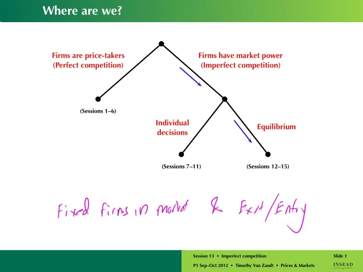
Where are we? Firms are price-takers Firms have market power (Perfect competition) (Imperfect competition) (Sessions 16) Individual Equilibrium decisions (Sessions 711) (Sessions 1215) Say: We did uniform pricing and price
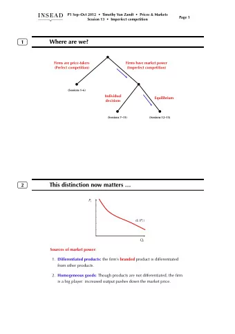
Where are we? Firms are price-takers Firms have market power (Perfect competition) (Imperfect competition) (Sessions 1–6) Individual Equilibrium decisions (Sessions 7–11) (Sessions 12–15) Say: We did uniform pricing and price discrimination at individual level, but we only bring uniform pricing to equilibrium. Session 13 • Imperfect competition Slide 1 P1 Sep–Oct 2012 • Timothy Van Zandt • Prices & Markets
This distinction now matters … P i d i ( P i ) Q i Sources of market power : 1. Differentiated products: the firm’s branded product is differentiated from other products. 2. Homogeneous goods: Though products are not differentiated, the firm is a big player: increased output pushes down the market price. Session 13 • Imperfect competition Slide 2 P1 Sep–Oct 2012 • Timothy Van Zandt • Prices & Markets
We begin with … Price competition with differentiated products Recall the pricing game from Session 12: Firm B Low Med High 19 18 10 Low 20 25 31 24 28 21 Med Firm A 23 31 38 30 40 34 High 15 27 42 We extend this to a full range of prices. Session 13 • Imperfect competition Slide 3 P1 Sep–Oct 2012 • Timothy Van Zandt • Prices & Markets
Let’s use the same story Recently appointed Recently appointed CEO of Firm A CEO of Firm B Session 13 • Imperfect competition Slide 4 P1 Sep–Oct 2012 • Timothy Van Zandt • Prices & Markets
Firm A’s pricing problem € 36 30 This is P ∗ 24 d A A “uniform pricing with market power” 18 MC A (Sessions 8 and 9). 12 6 Q A 20 40 60 80 100 Q ∗ A − 6 MR A Session 13 • Imperfect competition Slide 5 P1 Sep–Oct 2012 • Timothy Van Zandt • Prices & Markets
Nash equilibrium € € 36 36 30 30 P ∗ P ∗ 24 d A 24 d B A B 18 18 MC A MC B 12 12 6 6 Q A Q B 20 40 60 80 100 20 40 60 80 100 Q ∗ Q ∗ A B − 6 − 6 MR A MR B Session 13 • Imperfect competition Slide 6 P1 Sep–Oct 2012 • Timothy Van Zandt • Prices & Markets
Let’s use the numbers from Airbus-Boeing example Demand functions: Q A = 60 − 3 P A + 2 P B Q B = 60 − 3 P B + 2 P A Both firms have constant MC = 12 . Session 13 • Imperfect competition Slide 7 P1 Sep–Oct 2012 • Timothy Van Zandt • Prices & Markets
From the demand Some best responses … elasticity exercise Firm A’s demand curve when P B = 24 and when P B = 30 : P A P B = 30 ⇒ Q A = 120 − 3 P A 40 30 P B = 24 ⇒ Q A = 108 − 3 P A 20 10 30 60 90 120 Q A Session 13 • Imperfect competition Slide 8 P1 Sep–Oct 2012 • Timothy Van Zandt • Prices & Markets
In general: from Topic 9 on shifting demand … Higher price by Firm B Firm A ’s demand curve shifts … ⇒ Higher Volume? Lower Elasticity? up Firm A ’s profit-maximizing price goes ⇒ complements Thus, the pricing decisions are strategic Session 13 • Imperfect competition Slide 9 P1 Sep–Oct 2012 • Timothy Van Zandt • Prices & Markets
So remember, with price competition … When the goods are substitutes , the pricing decisions are strategic complements . (Holds for linear demand, and usually in the real world.) Session 13 • Imperfect competition Slide 10 P1 Sep–Oct 2012 • Timothy Van Zandt • Prices & Markets
Q A = 60 − 3 P A + 2 P B Firm A’s “residual” demand and best reply Constant MC = 12 When Firm B charges P B , Firm A ’s demand curve is: Q A = (60 + 2 P B ) − 3 P A ⇒ Firm A ’s choke price is: 20 + 2 3 P B ⇒ Firm A ’s optimal price is: 20 + 2 3 P B + 12 = 16 + 1 3 P B 2 Firm A ’s reaction curve: P A = 16 + 1 3 P B Session 13 • Imperfect competition Slide 11 P1 Sep–Oct 2012 • Timothy Van Zandt • Prices & Markets
Nash equilibrium Prices ( P ∗ A , P ∗ B ) such that: In words … As an equation … P A = 16 + 1 3 P B P ∗ A is a best response by firm A to P ∗ B P B = 16 + 1 3 P A P ∗ B is a best response by firm B to P ∗ A Session 13 • Imperfect competition Slide 12 P1 Sep–Oct 2012 • Timothy Van Zandt • Prices & Markets
Illustrating Nash equilibrium graphically P B 16 + 1 P A 3 P B = 55 16 + 1 P B 3 P A = 50 45 40 35 30 25 20 15 10 5 5 10 15 20 25 30 35 40 45 50 55 P A Session 13 • Imperfect competition Slide 13 P1 Sep–Oct 2012 • Timothy Van Zandt • Prices & Markets
Wrap up: Price competition with differentiated products 1. Each firm’s decision is same as “pricing with market power”: Topics 8&9. 2. Goods are substitutes ⇒ prices are strategic complements. (Always with linear demand; almost always in real life.) 3. Interaction captured by Nash equilibrium. Each firm’s price maximizes its own profit given price of the other firm. Session 13 • Imperfect competition Slide 14 P1 Sep–Oct 2012 • Timothy Van Zandt • Prices & Markets
Next we do … Quantity competition with homogeneous products Also called Cournot competition 1. Firms’ goods are perfect substitutes. 2. So firm doesn’t set price; it chooses how much to sell. 3. Market determines market-clearing price. 4. But each firm’s output decision affects this price. Session 13 • Imperfect competition Slide 15 P1 Sep–Oct 2012 • Timothy Van Zandt • Prices & Markets
Corning and glass substrate Corning has over 50% market share of glass substrate. There are different grades (“5G, 6G, …”), but for a particular grade the products of different suppliers are viewed as close substitutes. News item from December 2005 (for example): The aggressive capacity added by both Corning of the U.S., the world’s No. 1 substrate supplier, and AGC, the No. 2, will lead to price drops for glass substrates and will especially benefit TV panel makers … Session 13 • Imperfect competition Slide 16 P1 Sep–Oct 2012 • Timothy Van Zandt • Prices & Markets
Indonesian Cement Market Three major players: • 45%: Semen Gresik [State-owned] • 37%: Indocement [Owned by HeidelbergCement since 2001] • 17%: Holcim Indonesia [Owned by Holcim (Swiss) since 2006] Session 13 • Imperfect competition Slide 17 P1 Sep–Oct 2012 • Timothy Van Zandt • Prices & Markets
The protagonists Indocement Semen Gresik CEO of Indocement CEO of Semen Gresik Session 13 • Imperfect competition Slide 18 P1 Sep–Oct 2012 • Timothy Van Zandt • Prices & Markets
Nash equilibrium € € 36 36 30 30 P ∗ P ∗ 24 d 1 24 d 2 1 2 18 18 MC 1 MC 2 12 12 6 6 Q 1 Q 2 20 40 60 80 100 20 40 60 80 100 Q ∗ Q ∗ 2 1 − 6 − 6 MR 1 MR 2 Session 13 • Imperfect competition Slide 19 P1 Sep–Oct 2012 • Timothy Van Zandt • Prices & Markets
Market demand curve vs. Indocement’s demand curve MARKET DEMAND INDOCEMENT’S DEMAND Q = 1500 − 50 P When Q other = 500 P P 30 30 25 25 20 20 15 15 10 10 5 5 500 1000 1500 500 1000 1500 Q Q i Session 13 • Imperfect competition Slide 20 P1 Sep–Oct 2012 • Timothy Van Zandt • Prices & Markets
Indocement’s quantity decision (Constant MC = 10) When Q other = 200 When Q other = 500 P P 30 30 25 25 20 20 15 15 10 10 5 5 500 1000 1500 500 1000 1500 Q i Q i Session 13 • Imperfect competition Slide 21 P1 Sep–Oct 2012 • Timothy Van Zandt • Prices & Markets
Nash equilibrium Q 2 1000 800 600 400 200 Q 1 200 400 600 800 1000 Session 13 • Imperfect competition Slide 22 P1 Sep–Oct 2012 • Timothy Van Zandt • Prices & Markets
Wrap up: Quantity competition with homogeneous goods 1. Each firm’s output decision is same as “pricing with market power”: Topics 8&9. 2. Quantities are strategies substitutes. (Always with linear demand; almost always in real life.) 3. Use this model (rather than price competition) • for homogeneous products like oil, lycine, glass substrate, • to analyze investments in capacity. Session 13 • Imperfect competition Slide 23 P1 Sep–Oct 2012 • Timothy Van Zandt • Prices & Markets
Finally … Imperfect competition with exit/entry Session 13 • Imperfect competition Slide 24 P1 Sep–Oct 2012 • Timothy Van Zandt • Prices & Markets
Falafel vendors on the beach of Beirut h c a e B Session 13 • Imperfect competition Slide 25 P1 Sep–Oct 2012 • Timothy Van Zandt • Prices & Markets
See website for details, but you Numerical example: Cournot don’t have to be able to do this. • Market demand curve: Q = 1500 − 50 P • Constant MC = 10 . Then I calculate the Nash equilibrium for any number N of firms. Session 13 • Imperfect competition Slide 26 P1 Sep–Oct 2012 • Timothy Van Zandt • Prices & Markets
Recommend


More recommend
Explore More Topics
Stay informed with curated content and fresh updates.