Chapter 3: Price Discrimination A1. The goods produced by the - PDF document

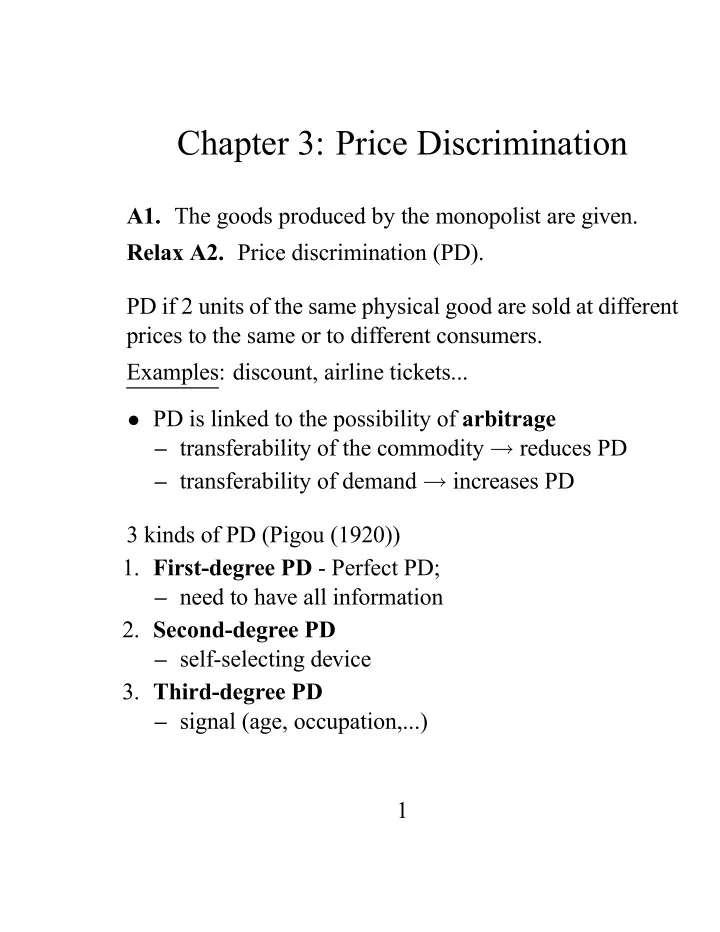
Chapter 3: Price Discrimination A1. The goods produced by the monopolist are given. Relax A2. Price discrimination (PD). PD if 2 units of the same physical good are sold at different prices to the same or to different consumers. Examples: discount, airline tickets... • PD is linked to the possibility of arbitrage – transferability of the commodity → reduces PD – transferability of demand → increases PD 3 kinds of PD (Pigou (1920)) 1. First-degree PD - Perfect PD; – need to have all information 2. Second-degree PD – self-selecting device 3. Third-degree PD – signal (age, occupation,...) 1

1 First Degree Price Discrimination • Discrete case – Identical consumers – unit demand – v : consumer’s willingness to pay. – A monopolist charges p = v in order to extract the entire surplus. • Continuous case – n identical consumers – same demand function q i = D ( p ) n – Total demand: q = D ( p ) – Linear pricing schedule T ( q ) = pq gives a pro fi t p m D ( p m ) − C ( D ( p m )) – The monopolist can increase his pro fi t if he proposes a two-part tariff : T ( q ) = A + pq. – The monopolist sets the competitive price p c . – The surplus of the consumers is Z q c S c = ( p ( q ) − p c ) dq 0 2

– And each consumer must pay a fi xed premium A = S c n – The monopolist proposes an af fi ne (nonlinear) pricing schedule ( two part tariff ): ( p c q + S c n if q > 0 T ( q ) = if q = 0 0 – The pro fi t of the monopolist is Π = S c + p c q − C ( q c ) • Non identical consumers: they have different demand curves. – The optimal pricing scheme is p = MC – and each consumer pays a personalized fi xed premium S c i ( p c ) . • BUT problem of information . • and of arbitrage.... 3

2 Third Degree PD • Single product, total cost C ( q ) • m groups of consumers (age, sex, occupation,...). • Each group has a different demand function. • Monopolist knows these demand functions. • No arbitrage between groups, but no PD within a group. • Linear tariff: { p 1 , ..., p i , ..., p m } • Quantities demanded: { q 1 = D 1 ( p 1 ) , ..., q i = D i ( p i ) , ..., q m = D m ( p m ) } • Aggregate demand is q = P m i =1 D i ( p i ) • Monopolist chooses prices that maximize m m X X D i ( p i ) p i − C ( D i ( p i )) i =1 i =1 • Remember: multiproduct pricing with independent demands and separable costs! ⇒ $ i ≡ p i − C 0 ( . ) = 1 p i ε i 4

Result 1 Optimal pricing implies that the monopolist should charge more in markets with the lower elasticity. Example: Students vs non-students... • What can we say in terms of welfare ? Does PD increase or decrease welfare? • What would happen if the monopolist were forced to charge the same price? Uniform price ( p ) Result 2 Consumers with high elastic demand (resp. low) prefer discrimination (resp. uniform pricing). • Marginal cost: c • Under PD: – p i in market i , D i ( p i ) = q i – Aggregate CS and pro fi t are m X CS D = S i ( p i ) i =1 X m Π m D = ( p i − c ) q i i =1 5

• PD is prohibited – uniform price p , and thus D i ( p ) = q i – Aggregate CS and pro fi t are X m CS No = S i ( p ) i =1 X m Π m No = ( p − c ) q i i =1 • Difference in total welfare ∆ W = CS D − CS No + Π m D − Π m No X m X m X m ∆ W = ( S i ( p i ) − S i ( p )) + ( p i − c ) q i − ( p − c ) q i i =1 i =1 i =1 • Thus – if ∆ W > 0 , welfare is higher under PD, – if ∆ W < 0 , welfare is lower under PD. 6

• Upper and lower bounds for ∆ W (to show) X m (1) ∆ W ≥ ( p i − c )( q i − q i ) i =1 m X (2) ∆ W ≤ ( p − c ) ( q i − q i ) i =1 • PD reduces welfare if it does not increase total output – from equation (2), if P m i =1 q i = P m i =1 q i then ∆ W ≤ 0 . • To be preferred socially, PD must raise total output. • Case of linear demand functions: q i = a i − b i p for i • Assume that a i > b i c for any i . • Under PD – Monopolist chooses p i that solves Max ( p i − c )( a i − b i p i ) 7

and thus p i = a i + cb i 2 b i q i = a i − cb i 2 – Thus the sum of the output is X m X m a i − cb i q i = 2 i =1 i =1 • Under uniform pricing – All markets are served at the optimum. – Monopolist chooses p that solves X m X m Max ( p − c )( a i − p b i ) i =1 i =1 and thus P m i =1 a i + c P m i =1 b i 2 P m p = i =1 b i P m i =1 a i − c P m X m i =1 b i q i = 2 i =1 8

• And thus, same total output m m m X X X q i = q i ⇒ ( q i − q i ) = 0 i =1 i =1 i =1 and according to equation (2) ∆ W ≤ 0 , welfare is lower under PD. • This outcome depends on the assumption: all markets are served under uniform pricing (+ linear demand). • Welfare conclusion can be reversed.... – 2 markets, i.e. m = 2 – under uniform pricing, second market is not served. – PD: p m 1 , p m 2 , q m 1 , q m 2 . – Uniform pricing: p = p m 1 , q 1 = q m 1 , q 2 = 0 , and thus X m ( q i − q i ) = q m 1 − q m 1 + q m 2 − 0 = q m 2 > 0 i =1 m X ( p i − c )( q i − q i ) = ( p m 1 − c ) × 0 + ( p m 2 − c ) q m 2 > 0 i =1 and from equation (1) ∆ W ≥ 0 . – In this case: PD increases welfare. – PD leads to Pareto improvement: monopolist makes more pro fi t, and CS increases in market 2. 9

• Ambiguous effects of PD on welfare . Trade-off between – loss of consumers in low-elasticity markets – gain of consumers in high-elasticity markets. • If PD is prohibited: it can conduct to closure of market.... 10

3 Second Degree PD • Heterogeneous consumers • Monopolist knows they are heterogeneous. • Monopolist will offer a menu of bundles to choose from. • Personal arbitrage can happen: self selection or incentive constraints. 3.1 Two Part Tariffs • T ( q ) = A + pq . • Menu of bundles { T, q } • Consumers’ preferences are ( θ V ( q ) − T if they pay T and consume q units u = otherwise 0 where – V (0) = 0 , V 0 ( q ) > 0 , V 00 ( q ) < 0 . – θ taste parameter. • 2 groups of consumers: – a proportion λ of consumers with parameter taste θ 1 ; – a proportion (1 − λ ) with parameter taste θ 2 . 11

• Marginal cost c, • Assumption: – θ 2 > θ 1 > c , – V ( q ) = 1 − (1 − q ) 2 and thus V 0 ( q ) = (1 − q ) > 0 2 • What is the demand function of a consumer θ i facing a price p ? – Consumer solves Max { θ i V ( q ) − pq } q – Thus demand function is D i ( p ) = 1 − p θ i – Aggregate demand function D ( p ) = λ D 1 ( p ) + (1 − λ ) D 2 ( p ) D ( p ) = 1 − p ( λ + 1 − λ ) = 1 − p θ 1 θ 2 θ where 1 θ = λ θ 1 + 1 − λ θ 2 is the “harmonic mean”. 12

– Net consumers surplus is S i ( p ) = θ i V ( D i ( p )) − pD i ( p ) S i ( p ) = ( θ i − p ) 2 2 θ i 3.1.1 Perfect Price Discrimination • If the monopolist can observe θ i • He charges p 1 = c per unit plus a fi xed premium A i = S i ( c ) = ( θ i − p 1 ) 2 2 θ i where ∂ A i ∂θ i > 0 , and thus A 2 > A 1 . • Pro fi t of the monopolist is Π 1 = λ ( θ 1 − p 1 ) 2 + (1 − λ )( θ 2 − p 1 ) 2 2 θ 1 2 θ 2 • If the monopolist cannot observe θ i : arbitrage problem. High demand consumers have an incentive to claim they are low demand type. 13

3.1.2 Monopoly Pricing • Monopolist charges a fully linear tariff T ( q ) = pq • Assumption: monopolist serves the two types of consumers (Formally c + θ 2 ≤ θ 1 and λ not too small). 2 • Monopolist chooses p that solves Max ( p − c ) D ( p ) p and thus p 2 = c + θ 2 and the monopolist pro fi t is Π 2 = ( θ − c ) 2 4 θ 3.1.3 Two-part tariff • Assumption: the monopolist serves the two-types of consumers. • To make them buy: A = S 1 ( p ) • Monopolist chooses p that solves Max { S 1 ( p ) + ( p − c ) D ( p ) } p 14

and thus the price is c p 3 = 2 − θ θ 1 and the pro fi t is Π 3 = S 1 ( p 3 ) + ( p 3 − c ) D ( p 3 ) 3.1.4 Comparison • Pro fi ts Π 1 ≥ Π 3 ≥ Π 2 – Maximum pro fi t under perfect PD – Monopolist can always duplicate a linear tariff with a two-part tariff. • Prices p 1 = c < p 3 < p 2 = p m – A lower price induces less monopoly pro fi t but higher fi xed part. • Welfare W ( p 3 ) > W ( p 2 ) as W ( p ) is decreasing with p . 15

W ( p ) = λ [ S g 1 ( p ) − cD 1 ( p )] + (1 − λ )[ S g 2 ( p ) − cD 2 ( p )] S g i ( p ) = S i ( p ) + pD i ( p ) S g i ( p ) = θ i V ( D i ( p )) − pD i ( p ) + pD i ( p ) S g i ( p ) = θ i V ( D i ( p )) Thus ∂ [ S g 1 ( p ) − cD 1 ( p )] = θ i V 0 ( p ) D 0 i ( p ) − cD 0 i ( p ) ∂ p = − p + c ≤ 0 θ i θ i – Because p 3 < p 2 , consumers under two part tariff consume more (reduces distortion) – And Π 3 ≥ Π 2 • Graph • Using a graph, show that for any linear tariff T ( q ) = pq with p > c , there exists a two-part tariff e pq + e T ( q ) = e A such that if consumers are offered the choice between T and e T , both types of consumers and the fi rm are made better off (exercise 3.4). 16