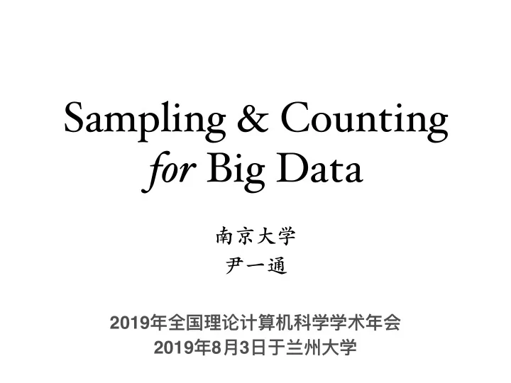
Sampling & Counting for Big Data 2019 - PowerPoint PPT Presentation

Sampling & Counting for Big Data ����� ��� 2019 �������������� 2019 � 8 � 3 ������

Sampling vs Counting for all self-reducible problems [Jerrum-Valiant-Vazirani ’86]: approx counting exact ( { approx } sampling vol( Ω ) Poly-Time approx inference X = ( X 1 , X 2 , …, X n ) Turing Machine X ∼ Ω Pr[ X i = ⋅ ∣ X S = σ ]

MCMC Sampling Markov chain for sampling X = ( X 1 , X 2 , …, X n ) ∼ μ • Gibbs sampling (Glauber dynamics, heat-bath) [Glauber, ’63] pick a random i ; [Geman, Geman, ’84] resample X i ~ µ v ( · | N ( v )) ; • Metropolis-Hastings algorithm pick a random i ; [Metropolis et al, ’53] propose a random c ; [Hastings, ’84] X i = c w.p. ∝ µ ( X’ )/ µ ( X ); • Analysis: coupling methods [Aldous , ’83] [Jerrum, ’95] [Bubley, Dyer ’97] may give O( n log n ) upper bound for mixing time

Computational Phase Transition hardcore model: graph G ( V , E ) , max-degree Δ , fugacity λ >0 approx sample independent set I in G w.p. ∝ λ | I | • λ c ( ∆ ) = ( ∆ − 1) ( ∆ − 1) [Weitz, STOC ’06] : If λ < λ c , n O(log Δ ) time. ( ∆ − 2) ∆ • [Sly, FOCS ’10 best paper] : If λ > λ c , λ 6 NP- hard even for Δ =O(1) . 5 Hard 4 3 [Efthymiou, Hayes, Š tefankovi č , 2 Easy Vigoda, Y., FOCS ’16]: 1 If λ < λ c , O( n log n ) mixing time. 2 4 6 8 10 max-deg Δ If Δ is large enough, and there is no small cycle. A phase transition occurs at λ c .

Big Data?

Sampling and Inference for Big Data • Sampling from a joint distribution (specified by a probabilistic graphical model ). • Inferring according to a probabilistic graphical model. • The data ( probabilistic graphical model ) is BIG.

• Parallel/distributed algorithms for sampling ? ✓ • PTIME ⟹ Polylog( n ) rounds • For parallel/distributed computing: ✓ sampling ≡ approx counting/inference ? • PTIME ⟹ Polylog( n ) rounds • Dynamic sampling algorithms ? ✓ • PTIME ⟹ Polylog( n ) incremental cost

Local Computation “ What can be computed locally? ” [Noar, Stockmeyer, STOC’93, SICOMP’95] the LOCAL model [Linial ’87] : • Communications are synchronized. • In each round: unlimited local computation and communication with neighbors. • Complexity: # of rounds to terminate in the worst case. • In t rounds: each node can collect information up to distance t . PLOCAL: t = polylog( n )

“What can be sampled locally?” • Joint distribution defined by local constraints: • Markov random field • Graphical model • Sample a random solution from the joint distribution: • distributed algorithms (in the LOCAL model) network G ( V , E ) Q: “What locally definable joint distributions are locally sample - able?”

MCMC Sampling Classic MCMC sampling: G ( V , E ): Markov chain X t → X t+ 1 : pick a uniform random vertex v ; v v update X ( v ) conditioning on X ( N ( v )) ; O( n log n ) time when mixing Parallelization: • Chromatic scheduler [folklore] [Gonzalez et al. , AISTAT’11] : Vertices in the same color class are updated in parallel. • O( Δ log n ) mixing time ( Δ is max degree) • “Hogwild!” [Niu, Recht, Ré, Wright, NIPS’11][De Sa, Olukotun, Ré, ICML’16] : All vertices are updated in parallel, ignoring concurrency issues. • Wrong distribution!

Crossing the Chromatic # Barrier Sequential Parallel O( n log n ) O( Δ log n ) parallel speedup = θ ( n / Δ ) ∆ = max-degree χ = chromatic no. Do not update adjacent vertices simultaneously. It takes ≥ χ steps to update all vertices at least once. Q: “How to update all variables simultaneously and still converge to the correct distribution?”

Markov Random Fields (MRF) μ ( σ ) ∝ ∏ ∀ σ ∈ [ q ] V : ∏ ν v ( σ v ) ϕ e ( σ u , σ v ) v ∈ V e =( u , v ) ∈ E • Each vertex v ∈ V : a variable over X v ∈ [ q ] ν v domain [ q ] with distribution ϕ e v u ν v • Each edge e =( u , v ) ∈ E : a symmetric binary constraint: ϕ e : [ q ] × [ q ] → [0,1] G ( V , E )

The Local-Metropolis Algorithm [Feng, Sun, Y., What can be sample locally ? PODC ’17] proposals: σ w σ u σ v u v w current: X u X v X w Markov chain X t → X t+ 1 : each vertex v ∈ V independently proposes a random ; σ v ∼ ν v each edge e =( u , v ) passes its check independently with prob: ϕ e ( X u , σ v ) ⋅ ϕ e ( σ u , X v ) ⋅ ϕ e ( σ u , σ v ); each vertex v ∈ V update X v to σ v if all its edges pass checks ; • Local-Metropolis converges to the correct distribution µ .

The Local-Metropolis Algorithm [Feng, Sun, Y., What can be sample locally ? PODC ’17] each vertex v ∈ V independently proposes a random ; σ v ∼ ν v each edge e =( u , v ) passes its check independently with prob: ϕ e ( X u , σ v ) ⋅ ϕ e ( σ u , X v ) ⋅ ϕ e ( σ u , σ v ); each vertex v ∈ V update X v to σ v if all its edges pass checks ; • Local-Metropolis converges to the correct distribution µ . μ ( σ ) ∝ ∏ MRF: ∏ ν v ( σ v ) ϕ e ( σ u , σ v ) v ∈ V e =( u , v ) ∈ E • under coupling condition for Metropolis-Hastings : • Metropolis-Hastings : O( n log n ) time • (lazy) Local-Metropolis : O(log n ) time

Lower Bounds [Feng, Sun, Y., What can be sample locally ? PODC ’17] Approx sampling from any MRF requires Ω (log n ) rounds. • for sampling: O(log n ) is the new criteria of “ local ” If λ > λ c , sampling from hardcore model requires Ω ( diam ) rounds. λ c ( ∆ ) = ( ∆ − 1) ( ∆ − 1) strong separation : sampling vs other ( ∆ − 2) ∆ local computation tasks λ 6 • Independent set is trivial to 5 construct locally (e.g. ∅ ). Hard 4 3 • The lower bound holds not because 2 Easy of the locality of information, but 1 because of the locality of correlation. 2 4 6 8 10 max-deg Δ

• Parallel/distributed algorithms for sampling ? ✓ • PTIME ⟹ Polylog( n ) rounds • For parallel/distributed computing: ✓ sampling ≡ approx counting/inference ? • PTIME ⟹ Polylog( n ) rounds • Dynamic sampling algorithms ? ✓ • PTIME ⟹ Polylog( n ) incremental cost

Example : Sample Independent Set (hardcore model) µ : distribution of independent sets I in G ∝ λ | I | • Y ∈ {0,1} V indicates an independent set • Each v ∈ V returns a Y v ∈ {0,1} , such that Y = ( Y v ) v ∈ V ∼ µ • Or: d TV ( Y , µ ) < 1/poly( n ) network G ( V , E )

Inference (Local Counting) µ : distribution of independent sets I in G ∝ λ | I | : marginal distribution at v conditioning on σ ∈ {0,1} S . µ σ v ∀ y ∈ { 0 , 1 } : v ( y ) = Pr Y ∼ µ [ Y v = y | Y S = σ ] µ σ 0 • Each v ∈ S receives σ v as input. • Each v ∈ V returns a marginal 0 distribution such that: µ σ ˆ v 1 1 1 d TV (ˆ v ) ≤ µ σ v , µ σ poly( n ) n 1 Y Z = µ ( ∅ ) = Y ∼ µ [ Y v i = 0 | ∀ j < i : Y v j = 0] Pr network G ( V , E ) i =1 Z : partition function (counting)

Decay of Correlation : marginal distribution at v conditioning on σ ∈ {0,1} S . µ σ v strong spatial mixing (SSM): ∀ boundary condition B ∈ {0,1} r -sphere( v ) : v , µ σ ,B d TV ( µ σ ) ≤ poly( n ) · exp( − Ω ( r )) v SSM (iff λ ≤ λ c when µ is the G hardcore model) r approx. inference is solvable v B in O(log n ) rounds σ in the LOCAL model

Locality of Counting & Sampling [Feng, Y., PODC ’18] For all self-reducible graphical models: Inference: Sampling: Correlation Decay: local approx. local approx. SSM inference sampling easy with additive error O(log 2 n ) factor local approx. local exact inference sampling with multiplicative error distributed Las Vegas sampler

Locality of Sampling Inference: Sampling: Correlation Decay: local approx. local approx. SSM inference sampling return a random Y = ( Y v ) v ∈ V each v can compute a µ σ ˆ v within O(log n ) -ball whose distribution ˆ µ ≈ µ 1 s.t. 1 d TV (ˆ µ, µ ) ≤ d TV (ˆ v ) ≤ µ σ v , µ σ poly( n ) poly( n ) sequential O(log n ) -local procedure: • scan vertices in V in an arbitrary order v 1 , v 2 , …, v n • for i =1,2, …, n : sample according to Y v 1 ,...,Y vi − 1 Y v i ˆ µ v i

Network Decomposition ( C , D ) -network-decomposition of G : • classifies vertices into clusters; • assign each cluster a color in [ C ] ; • each cluster has diameter ≤ D ; • clusters are properly colored. ( C , D ) r -ND: ( C , D ) -ND of G r Given a ( C , D ) r - ND: sequential r -local procedure: r = O(log n ) r = O(log n ) • scan vertices in V in an arbitrary order v 1 , v 2 , …, v n • for i =1,2, …, n : sample according to Y v 1 ,...,Y vi − 1 Y v i ˆ µ v i can be simulated in O( CDr ) rounds in LOCAL model

Network Decomposition ( C , D ) -network-decomposition of G : • classifies vertices into clusters; • assign each cluster a color in [ C ] ; • each cluster has diameter ≤ D ; • clusters are properly colored. ( C , D ) r -ND: ( C , D ) -ND of G r ( O(log n ), O(log n )) r -ND can be constructed in O( r log 2 n ) rounds w.h.p. [Ghaffari, Kuhn, Maus, STOC’17]: r -local SLOCAL algorithm: O( r log 2 n ) -round LOCAL alg.: ND ∀ ordering π =( v 1 , v 2 , …, v n ) , returns w.h.p. the Y ( π ) for some ordering π returns random vector Y ( π )