Sampling and Sample Size Rohit Naimpally J-PAL Course Overview 1. - PowerPoint PPT Presentation
YEF ITCILO - JPAL Evaluating Youth Employment Programmes: An Executive Course 22 26 June 2015 ITCILO Turin, Italy Sampling and Sample Size Rohit Naimpally J-PAL Course Overview 1. Introduction to Impact Evaluation 2. Measurement
N = 10 N = 50 Frequency of Means With 5 Samples Frequency of Means With 5 Samples 10 10 8 8 6 6 4 4 2 2 0 0 1 3 5 7 9 11 13 15 17 19 21 23 25 27 29 31 33 35 37 39 41 43 45 47 49 51 1 3 5 7 9 11 13 15 17 19 21 23 25 27 29 31 33 35 37 39 41 43 45 47 49 51 Frequency of Means With 10 Samples Frequency of Means With 10 Samples 10 10 9 9 8 8 7 7 6 6 5 5 4 4 3 3 2 2 1 1 0 0 1 3 5 7 9 11 13 15 17 19 21 23 25 27 29 31 33 35 37 39 41 43 45 47 49 51 1 3 5 7 9 11 13 15 17 19 21 23 25 27 29 31 33 35 37 39 41 43 45 47 49 51
N = 10 N = 50 Frequency of Means With 50 Samples Frequency of Means With 50 Samples 14 14 12 12 10 10 8 8 6 6 4 4 2 2 0 0 1 3 5 7 9 11 13 15 17 19 21 23 25 27 29 31 33 35 37 39 41 43 45 47 49 51 1 3 5 7 9 11 13 15 17 19 21 23 25 27 29 31 33 35 37 39 41 43 45 47 49 51 Frequency of Means With 100 Frequency of Means with 100 Samples Samples 20 20 15 15 10 10 5 5 0 0 1 3 5 7 9 11 13 15 17 19 21 23 25 27 29 31 33 35 37 39 41 43 45 47 49 51 1 3 5 7 9 11 13 15 17 19 21 23 25 27 29 31 33 35 37 39 41 43 45 47 49 51
N = 10 N = 50 Frequency of Means With 500 Frequency of Means With 500 Samples Samples 90 100 80 70 60 50 40 30 20 10 0 -10 1 3 5 7 9 11 13 15 17 19 21 23 25 27 29 31 33 35 37 39 41 43 45 47 49 51 1 3 5 7 9 11 13 15 17 19 21 23 25 27 29 31 33 35 37 39 41 43 45 47 49 51 Frequency of Means With 1000 Frequency of Means With 1000 Samples Samples 160 200 150 110 100 60 50 10 0 1 3 5 7 9 11 13 15 17 19 21 23 25 27 29 31 33 35 37 39 41 43 45 47 49 51 1 3 5 7 9 11 13 15 17 19 21 23 25 27 29 31 33 35 37 39 41 43 45 47 49 51 -40
Outline • Sampling distributions – population distribution – sampling distribution – law of large numbers/central limit theorem – standard deviation and standard error • Detecting impact
Population & sampling distribution: Draw 1 random student (from 8,000) 500 4.0% 450 3.5% 400 3.0% 350 2.5% 300 mean 26 250 2.0% frequency 200 1.5% freq (N=1) 150 1.0% 100 0.5% 50 0 0.0% 0 5 10 15 20 25 30 35 40 45 50 55 60 65 70 75 80 85 90 95 100 test scores
Sampling Distribution: Draw 4 random students (N=4) 500 4.5% 450 4.0% 400 3.5% 350 3.0% 300 2.5% mean 26 250 frequency 2.0% 200 freq (N=4) 1.5% 150 1.0% 100 0.5% 50 0 0.0% 0 5 10 15 20 25 30 35 40 45 50 55 60 65 70 75 80 85 90 95 100 test scores
Law of Large Numbers : N=9 500 7.0% 450 6.0% 400 5.0% 350 300 4.0% mean 26 250 frequency 3.0% 200 freq (N=9) 150 2.0% 100 1.0% 50 0 0.0% 0 5 10 15 20 25 30 35 40 45 50 55 60 65 70 75 80 85 90 95 100 test scores
Law of Large Numbers: N =100 500 25.0% 450 400 20.0% 350 300 15.0% mean 26 250 frequency 200 10.0% freq (N=100) 150 100 5.0% 50 0 0.0% 0 5 10 15 20 25 30 35 40 45 50 55 60 65 70 75 80 85 90 95 100 test scores
Central Limit Theorem: N=1 500 4.0% 450 3.5% 400 3.0% 350 2.5% 300 mean 26 250 2.0% frequency dist_1 200 1.5% freq (N=1) 150 1.0% 100 0.5% 50 0 0.0% 0 5 10 15 20 25 30 35 40 45 50 55 60 65 70 75 80 85 90 95 100 test scores The white line is a theoretical distribution
Central Limit Theorem : N=4 500 4.5% 450 4.0% 400 3.5% 350 3.0% 300 mean 2.5% 26 250 frequency 2.0% dist_4 200 freq (N=4) 1.5% 150 1.0% 100 0.5% 50 0 0.0% 0 5 10 15 20 25 30 35 40 45 50 55 60 65 70 75 80 85 90 95 100 test scores
Central Limit Theorem : N=9 500 7.0% 450 6.0% 400 5.0% 350 300 4.0% mean 26 250 frequency 3.0% dist_9 200 freq (N=9) 150 2.0% 100 1.0% 50 0 0.0% 0 5 10 15 20 25 30 35 40 45 50 55 60 65 70 75 80 85 90 95 100 test scores
Central Limit Theorem : N =100 500 25.0% 450 400 20.0% 350 300 15.0% mean 26 250 frequency dist_100 200 10.0% freq (N=100) 150 100 5.0% 50 0 0.0% 0 5 10 15 20 25 30 35 40 45 50 55 60 65 70 75 80 85 90 95 100 test scores
So Why Do We Care? • Sampling distribution is a probability distribution • Sampling Distribution is a bell curve ( irrespective of what the underlying distribution is) • Why does it matter? • Why do we care if the probability distribution looks like a bell curve? • Because we know how to calculate the area underneath!
95% Confidence Interval 0.5 0.45 0.4 0.35 0.3 0.25 0.2 0.15 0.1 0.05 0 -4 -3 -2 -1 0 1 2 3 4 5 6 1.96 SD 1.96 SD
Outline • Sampling distributions – population distribution – sampling distribution – law of large numbers/central limit theorem – standard deviation and standard error • Detecting impact
Standard deviation/error • But wait! The regression results that I have seen typically report the standard error , not the standard deviation . • What’s the difference between the standard deviation and the standard error? The standard error = the standard deviation of the sampling distribution
Variance and Standard Deviation • Variance = 400 𝜏 2 = 𝑃𝑐𝑡𝑓𝑠𝑤𝑏𝑢𝑗𝑝𝑜 𝑊𝑏𝑚𝑣𝑓 − 𝐵𝑤𝑓𝑠𝑏𝑓 2 𝑂 • Standard Deviation = 20 𝜏 = 𝑊𝑏𝑠𝑗𝑏𝑜𝑑𝑓 • Standard Error = 20 𝑂 SE = 𝜏 𝑂
Standard Deviation/ Standard Error 500 4.0% 450 3.5% 400 3.0% 350 2.5% 300 mean frequency 26 250 2.0% sd 200 1.5% dist_1 150 1.0% 100 0.5% 50 0 0.0% 0 5 10 15 20 25 30 35 40 45 50 55 60 65 70 75 80 85 90 95 100 test scores
Sample size ↑ x4, SE ↓ ½ 500 4.5% 450 4.0% 400 3.5% 350 3.0% 300 mean 2.5% 26 frequency 250 2.0% sd 200 se4 1.5% 150 dist_4 1.0% 100 0.5% 50 0 0.0% 0 5 10 15 20 25 30 35 40 45 50 55 60 65 70 75 80 85 90 95 100 test scores
Sample size ↑ x9, SE ↓ ? 500 7.0% 450 6.0% 400 5.0% 350 300 4.0% mean 26 250 frequency sd 3.0% 200 se9 dist_9 150 2.0% 100 1.0% 50 0 0.0% 0 5 10 15 20 25 30 35 40 45 50 55 60 65 70 75 80 85 90 95 100 test scores
Sample size ↑ x100, SE ↓? 500 25.0% 450 400 20.0% 350 300 15.0% mean frequency 26 250 sd 200 10.0% se100 dist_100 150 100 5.0% 50 0 0.0% 0 5 10 15 20 25 30 35 40 45 50 55 60 65 70 75 80 85 90 95 100 test scores
Outline • Sampling distributions • Detecting impact – significance – effect size – power – baseline and covariates – clustering – stratification
Baseline test scores 500 450 400 350 300 250 200 150 100 50 0 0 5 10 15 20 25 30 35 40 45 50 55 60 65 70 75 80 85 90 95 100 test scores
We implement the Balsakhi Program
Endline test scores 160 140 120 100 80 60 40 20 0 0 5 10 15 20 25 30 35 40 45 50 55 60 65 70 75 80 85 90 95 100 test scores After the balsakhi programs, these are the endline test scores
The impact appears to be? 500 A. Positive 400 300 B. Negative 200 C. No impact 100 0 0 5 10 15 20 25 30 35 40 45 50 55 60 65 70 75 80 85 90 95 100 D. Don’t know Baseline test scores 160 140 120 100 80 60 40 20 0 0 5 10 15 20 25 30 35 40 45 50 55 60 65 70 75 80 85 90 95 100 Endline test scores
Post-test: control & treatment 160 140 120 100 control 80 treatment 60 40 20 0 0 5 10 15 20 25 30 35 40 45 50 55 60 65 70 75 80 85 90 95 100 test scores Stop! That was the control group. The treatment group is red.
Is this impact statistically significant? 160 Average Difference = 6 points 140 120 100 control 80 treatment 60 control μ 40 treatment μ 20 0 0 5 10 15 20 25 30 35 40 45 50 55 60 65 70 75 80 85 90 95 100 test scores A. Yes B. No C. Don’t know
One experiment: 6 points
One experiment
Two experiments
A few more…
A few more…
Many more…
A whole lot more…
…
Running the experiment thousands of times… By the Central Limit Theorem, these are normally distributed
The assumption about your sample The Central Limit Theorem and the Law of Large Numbers hold if the sample is randomly sampled from your population
Theoretical Sampling distribution 0.5 0.45 0.4 0.35 0.3 0.25 0.2 0.15 0.1 0.05 0 -4 -3 -2 -1 0 1 2 3 4 5 6
So let’s look at hypothesis testing • In criminal law, most institutions follow the rule: “ innocent until proven guilty ” • In program evaluation, instead of “presumption of innocence,” the rule is: “presumption of insignificance” • The “ Null hypothesis ” ( H 0 ) is that there was no (zero) impact of the program • The burden of proof is on the evaluator to show a significant difference – Think about how this relates to the discussion of ethics on Sunday.
Hypothesis testing: conclusions • If it is very unlikely ( less than a 5% probability ) that the difference is solely due to chance: – We “reject our null hypothesis” • We may now say: – “our program has a statistically significant impact ”
Hypothesis Testing: Steps 1. Determine the (size of the) sampling distribution around the null hypothesis H 0 by calculating the standard error 2. Choose the confidence interval, e.g. 95% (or significance level: α ) ( α =5%) 3. Identify the critical value (boundary of the confidence interval) 4. If our observation falls in the critical region we can reject the null hypothesis
Remember our 95% Confidence Interval? 0.5 H 0 0.45 0.4 0.35 0.3 0.25 control 0.2 0.15 0.1 0.05 0 -4 -3 -2 -1 0 1 2 3 4 5 6 1.96 SD 1.96 SD
Impose significance level of 5% 0.5 H 0 H 0 H 0 0.45 0.4 0.35 0.3 0.25 control 0.2 0.15 0.1 0.05 0 -4 -3 -2 -1 0 1 2 3 4 5 6 1.96 SD
What is the significance level? • Type I error: rejecting the null hypothesis even though it is true (false positive) • Significance level: The probability that we will reject the null hypothesis even though it is true
What is Power? • Type II Error: Failing to reject the null hypothesis (concluding there is no difference), when indeed the null hypothesis is false. • Power: If there is a measureable effect of our intervention (the null hypothesis is false), the probability that we will detect an effect (reject the null hypothesis)
Hypothesis testing: 95% confidence YOU CONCLUDE CLUDE Effective No Effect Type e II Error or (low power) Effective THE Type e I Error TRUTH TH (5% of the time) No Effect
Before the experiment 0.5 0.45 0.4 0.35 0.3 H β control 0.25 H 0 0.2 treatment 0.15 0.1 0.05 0 -4 -3 -2 -1 0 1 2 3 4 5 6 Assume two effects: no effect and treatment effect β
Impose significance level of 5% 0.5 0.45 0.4 0.35 H 0 0.3 H β control Type I Error 0.25 treatment 0.2 significance 0.15 0.1 0.05 0 -4 -3 -2 -1 0 1 2 3 4 5 6 Anything between lines cannot be distinguished from 0
Can we distinguish H β from H0 ? 0.5 0.45 Type II Error 0.4 0.35 0.3 control H β 0.25 H 0 treatment 0.2 power 0.15 0.1 0.05 0 -4 -3 -2 -1 0 1 2 3 4 5 6 Shaded area shows % of time we would find H β true if it was
What influences power? • What are the factors that change the proportion of the research hypothesis that is shaded — i.e. the proportion that falls to the right (or left) of the null hypothesis curve? • Understanding this helps us design more powerful experiments.
Power: main ingredients 1. Sample Size (N) 2. Effect Size ( δ ) 3. Variance ( σ ) 4. Proportion of sample in T vs. C 5. Clustering ( ρ ) 6. Non-Compliance (akin to δ↓)
Power: main ingredients 1. Sample Size (N) 2. Effect Size ( δ ) 3. Variance ( σ ) 4. Proportion of sample in T vs. C 5. Clustering ( ρ ) 6. Non-Compliance (akin to δ↓)
By increasing sample size you increase… 0.5 0.45 0.4 0.35 0.3 control 0.25 treatment 0.2 power 0.15 0.1 0.05 0 -4 -3 -2 -1 0 1 2 3 4 5 6 A. Accuracy B. Precision C. Both D. Neither E. Don’t know
Power: Effect size = 1SE, Sample size = N 0.5 0.45 0.4 0.35 0.3 control 0.25 treatment 0.2 significance 0.15 0.1 0.05 0 -4 -3 -2 -1 0 1 2 3 4 5 6 Remember, your sampling distribution becomes narrower as N ↑
Power: Sample size = 4N 0.5 0.45 0.4 0.35 0.3 control 0.25 treatment 0.2 significance 0.15 0.1 0.05 0 -4 -3 -2 -1 0 1 2 3 4 5 6
Power: 64% 0.5 0.45 0.4 0.35 0.3 control 0.25 treatment 0.2 power 0.15 0.1 0.05 0 -4 -3 -2 -1 0 1 2 3 4 5 6
Power: Sample size = 9N 0.5 0.45 0.4 0.35 0.3 control 0.25 treatment 0.2 significance 0.15 0.1 0.05 0 -4 -3 -2 -1 0 1 2 3 4 5 6
Power: 91% 0.5 0.45 0.4 0.35 0.3 control 0.25 treatment 0.2 power 0.15 0.1 0.05 0 -4 -3 -2 -1 0 1 2 3 4 5 6
Recommend
More recommend
Explore More Topics
Stay informed with curated content and fresh updates.
