Sage Quick Reference: Statistics Max: v= list v.max() or - PowerPoint PPT Presentation

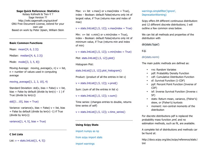
Sage Quick Reference: Statistics Max: v= list v.max() or v.max(index = True), warnings.simplefilter('ignore', Kelsey Kofmehl & Tien-Y ? index – Boolean: default False(returns only int of DeprecationWarning) Sage Version ?? largest value, if True (returns max and index of http://wiki.sagemath.org/quickref Scipy offers 84 different continuous distributions max) GNU Free Document License, extend for your and 12 different discrete distributions; I will own use v = stats.IntList([1,5, 12]); v.max(index = True) outline a few common ones below. Based on work by Peter Jipsen, William Stein Min: v= list v.min() or v.min(index = True), We can list all methods and properties of the index – Boolean: default False(returns only int of distribution with minimum value, if True (returns min and index Basic Common Functions dir(stats.’type’) of min) Mean: mean([4, 6, 2.3]) e.g. v = stats.IntList([1,5, 12]); v.min(index = True) Median: median([4, 6, 2.3]) dir(stats.norm) Plot: stats.IntList([1,5, 12]).plot() Mode: mode([3, 3, 5, 8]) The main public methods are defined as: Histogram Plot: Moving Average: moving_average(v, n) v = list, rvs: Random Variates • stats.IntList([1,5, 12]).plot_histogram() n = number of values used in computing pdf: Probability Density Function • average Product: (product of all the entries in list v) cdf: Cumulative Distribution Function • sf: Survival Function (1-CDF) • moving_average([1, 2, 3, 10], 4) v = stats.IntList([1,5, 12]); v.prod() ppf: Percent Point Function (Inverse of • CDF) Standard Deviation: std(v, bias = False) v = list, Sum: (sum of all the entries in list v) bias = False by default (divide by len(v) – 1 ) if isf: Inverse Survival Function (Inverse of • SF) True (divide by len(v)) v = stats.IntList([1,5, 12]); v.sum() stats: Return mean, variance, (Fisher’s) • std([1…10], bias = True) Time series: (changes entries to double, returns skew, or (Fisher’s) kurtosis time series of self) moment: non-central moments of the • Variance: variance(v, bias = False) v = list, bias distribution = False by default (divide by len(v) -1) if True v = stats.IntList([1,5, 12]); v.time_series() (divide by len(v)) For discrete distributions pdf is replaced the probability mass function pmf , and no variance([1, 4, 5], bias = True) estimation methods, such as fit, are available. Using Scipy Stats A complete list of distributions and methods can import numpy as np be found at: C Int Lists from scipy import stats http://docs.scipy.org/doc/scipy/reference/stats.h List: v = stats.IntList([1, 4, 5]) tml import warnings

def _pdf: computed o ... stats.cmedian(a[, numbins]) Continuous Distributions ... a = array, numbins = number of bins used to (take the loc and scale as keyword parameters histogram the data to adjust location and size of distribution e.g. for the standard normal distribution location is the stats.cmedian([2, 3, 5, 6, 12, 345, 333], 2) mean and scale is the standard deviation) Discrete Distributions Trimmed o Common types of continuous: (The location parameter, keyword loc can be stats.tmean( a , limits=None , inclusive=(True , used to shift the distribution) Normal • True) ) from scipy.stats import norm Common types of discrete: numargs = norm.numargs Harmonic o [ ] = [0.9,] * numargs Bernoulli • rv = norm() stats.hmean( a , axis=0 , dtype=None ) from scipy.stats import bernoulli [ pr ] = [<Replace with reasonable Skew • Cauchy • values>] from scipy.stats import cauchy rv = bernoulli(pr) stats.skew( a , axis=0 , bias=True) numargs = cauchy.numargs [ ] = [0.9,] * numargs Poisson • Signal to noise ratio • rv = cauchy() from scipy.stats import poisson stats.signaltonoise( a , axis=0 , ddof=0) [ mu ] = [<Replace with reasonable Expontential • values>] • Standard error of the mean from scipy.stats import expon rv = poisson(mu) numargs = expon.numargs stats.sem( a , axis=0 , ddof=1 ) [ ] = [0.9,] * numargs rv = expon() Historgram • Statistical Functions: stats.histogram2( a , bins ) Means: • To create a continuous class we use the base Geometric o Relative Z- scores • class rv_continuous: stats.gmean(a, axis, dtype) stats.zmap( scores , compare , axis=0 , ddof=0 e.g. a = array, axis = default 0, axis along which Z-score of each value • class gaussian_gen(stats.rv_continuous): geometric mean is computed, dtype = type of stats.zscore( a , axis=0 , ddof=0 ) "Gaussian distribution" returned array Regression line • You can then go on to define the parameters of stats.gmean([1,4, 6, 2, 9], axis=0, dtype=None) methods:

stats.linregress( x , y=None) stats.ppcc_max( x , brack=(0.0 , 1.0) , dist='tukeylambda' x = np.random.random(20) Ppcc (Returns (shape, ppcc), and • y = np.random.random(20) optionally plots shape vs. ppcc (probability plot correlation coefficient) slope, intercept, r_value, p_value, std_err = as a function of shape parameter for a stats.linregress(x,y) one-parameter family of distributions from shape value a to b.) For a complete list see ‘Statistical Functions”: http://docs.scipy.org/doc/scipy/reference/stats.h stats.ppcc_plot( x , a , b , dist='tukeylambda' , tml plot=None , N=80 Models Linear model fit • Markov Models: stats.glm( data , para ) Plots Probability plot • stats.probplot( x , sparams=() , dist='norm' , fit=True , plot=None ) x = array, sample response data, sparams = tuple, optional, dist = distribution function name (default = normal), fit = Boolean (default true) fit a least squares regression line to data, plot = plots the least squares and quantiles if given. stats.probplot([6, 23, 6, 23, 15, 6, 32, 1], sparams=(), dist='norm', fit=True, plot=None) Ppcc max (Returns the shape parameter • that maximizes the probability plot correlation coefficient for the given data to a one-parameter family of distributions)