S. Uhlenbrook, J.W. Foppen, I. Masih, S. Maskey, C. Orup, A. - PowerPoint PPT Presentation
20-23 September 2010, HydroPredict 2010 , 2nd Intern. Interdisciplinary Conference on Predictions for Hydrology, Ecology, and Water Resources Management: Changes and Hazards caused by Direct Human Interventions and Climate Change; Prague,
20-23 September 2010, HydroPredict ’ 2010 , 2nd Intern. Interdisciplinary Conference on Predictions for Hydrology, Ecology, and Water Resources Management: Changes and Hazards caused by Direct Human Interventions and Climate Change; Prague, Czech Republic Predicting the Impact of Change – The need for a better hydrological process understanding through innovative experimental and modeling approaches S. Uhlenbrook, J.W. Foppen, I. Masih, S. Maskey, C. Orup, A. Saraiva, V. Smakthin, J. Wenninger
Outlin Ou line (1) Intro the world is changing (‘ stationary is dead ’ ) (2) Case study ONE: Improving hydrological predictions in the semi-arid Karkheh basin, Iran (3) Case study TWO: DNA – New multi-tracing opportunities to study hydrological flow pathways (4) Case study THREE: The use of stable isotopes to improve our understanding of evaporation fluxes
6 High Risk for Instabilities 5 IPCC Projections 2100 AD Global Temperature ( ° C) It is Getting 4 Warmer! 3 The context – 2 Lower Risk for Instabilities ONE N.H. Temperature ( ° C) 1 1 0.5 0 0 -0.5 (NEAA, 2009) 1000 1200 1400 1600 1800 2000
Climate Sensitivity – Best estimate +3C for 2x CO 2 pre- industrial, but it can be much higher … (NEAA, 2009)
Change in annual runoff by 2041-60 (SRES A1B) – Ensemble of 12 climate models Source: Kundzewicz et al. (2007); chapter in IPCC (2007)
The context – TWO A massive land-grabbing scramble in Africa as foreign companies - some with foreign aid money support - rapidly establish enormous monoculture fields in tropical countries. Prof Seif Madoffe, SUA Sugar Cane – Kilombera Basin, 'climate colonialism' Tanzania
Impact of land use change on P P hydrological processes E I P E S E T E I P E S E T S S S S Q R Q R Q S Q R Q R Q S Short-term dynamics (e.g. interception, flood generation) vs. long-term dynamics (e.g. groundwater recharge, base flow) Picture from Fairless, 2007, Nature
Water Balance Equation: dS dS dS dS g I E s E Q u E E Q Q P dt dt dt dt I s s T u f g Where: dS E I Interception processes dt I dS s E Q Surface water processes dt s s dS E E Q u Root zone moisture processes dt T u f dS g Q Groundwater processes g dt Possible changes in all variables due to climate and/or land changes!!
Global Changes Climate (temperature, precipitation, radiation …) Land use, land cover De-forestation / re-forestation Urbanisation Etc. Population (amount, density, structure, …) Hydraulic works Technological development Globalisation Water use in space and time Economic development Change of diet (more meat => more water) N- and P-fluxes to water bodies Pollution (new substances etc.) Change in composition of species etc. etc. etc. …. and many interdependencies/feedbacks!
Why is it so difficult to predict hydrological effects of change? 1. Many global changes occur simultaneously with positive or negative (unknow) feedbacks 2. Spatial and temporal scales for hydrological processes are different from scales dominant in other disciplines 3. Hydrological processes are often non-linear or depend on thresholds/tipping points 4. Hydrological extremes (e.g. floods and droughts) do not occur often and are difficult to measure, consequently, good data sets are usually not available 5. Boundary conditions during hydrological modelling are not clear (i.e. subsurface flows) 6. Hydrological observation methods are insufficient to study hydrological process dynamics (e.g. subsurface flow processes, extreme events etc.)
Outlin Ou line (1) Intro the world is changing (‘ stationary is dead ’ ) (2) Case study ONE: Improving hydrological predictions in the semi-arid Karkheh basin, Iran (3) Case study TWO: DNA – New multi-tracing opportunities to study hydrological flow pathways (4) Case study THREE: The use of stable isotopes to improve our understanding of evaporation fluxes
The Karkheh basin, Iran Some basic facts and figures Drainage area: 50,764 km 2 More than 80 % is mountainous Divided into five sub-basins Mediterranean climate: Cool and wet winter; dry and hot summers Precipitation 450 mm/year, range: 150 mm to 750 mm Water allocations in 2001 Water allocations in 2025 (4949 MCM) (8903 MCM) Others, 14 Others, 512 Domestic, 362 Domestic, 262 Environment, Environment, Industry, 113 Industry, 23 500 500 Irrigation, 7416 Source: JAMAB 2006 Irrigation, 4149
Improving precipitation input in rainfall- runoff modeling using SWAT The current way of climatic data input in SWAT is rather simple One station nearest to the centroid of a catchment Gauge nearest to the centroid may not be the best representative This can undermine the full use of available data (e.g. if two stations in a sub-catchment, only one will be used) Quality of the climatic data input will has serious implications for the model parameterization and quality of (spatial and temporal) the results
Preparation of areal precipitation input 1) Rain gauge data 2) Gauge location 3) DEM /Elevation 4) Sub-basin ID Interpolation using IDW including elevation weighting Cross validation Areal average for sub-catchment Virtual rain gauge data Input for each sub-catchment Masih et al., JAWRA; in review
Comparison of the input precipitation: Case II (areal precipitation) vs. Case I (station data): Spatial view Sub-catchment precipitation Precipitation difference (Case II vs. Case 1) (Case II) High spatial variability, mainly influenced by topography (left) The precipitation difference in Case II compared to Case I ranged from -40 to 40 % (right)
Comparison Case II vs. Case I: Daily Monthly Annual Sub-catchment ID: 33 Sub-catchment ID: 33 Sub-catchment ID: 33 Temporal view 1000 300 100 P Case I (mm/month) P Case I (mm/year) P Case I (mm/day) 250 800 80 200 600 60 150 400 40 100 200 20 50 Divergent variations by sub-catchment, 0 0 0 0 200 400 600 800 1000 0 50 100 150 200 250 300 0 20 40 60 80 100 illustrated by four selected cases. P Case II (mm/year) P Case II (mm/month) P Case II (mm/day) Sub-catchment ID: 43 Precipitation dynamics in Case II could Sub-catchment ID: 43 Sub-catchment ID: 43 100 1000 300 P Case I (mm/month) P Case I (mm/day) P Case I (mm/year) 250 80 800 be different in many respects. 200 60 600 150 40 400 100 20 200 Daily values can be higher/lower. They 50 0 0 0 0 20 40 60 80 100 0 50 100 150 200 250 300 0 200 400 600 800 1000 also show clear pattern in extreme P Case II (mm/day) P Case II (mm/month) P Case II (mm/year) values: Sub-catchment ID: 1 Sub-catchment ID: 1 Sub-catchment ID: 1 100 300 1000 P Case I (mm/month) P Case I (mm/day) P Case I (mm/year) 250 80 800 1) lower P events can be totally missed 200 60 600 150 out be a single rain gauge; 40 400 100 20 200 50 0 0 0 2) extremes in Case II are 0 20 40 60 80 100 0 50 100 150 200 250 300 0 200 400 600 800 1000 P Case II (mm/day) P Case II (mm/month) P Case II (mm/year) comparatively small in most cases, Sub-catchment ID: 63 Sub-catchment ID: 63 Sub-catchment ID: 63 though could be other way around 1600 120 350 P Case I (mm/month) P Case I (mm/day) P Case I (mm/year) 300 100 1200 for some sub-catchments and P 250 80 200 800 60 150 events. 40 100 400 20 50 0 0 0 0 50 100 150 200 250 300 350 0 400 800 1200 1600 0 20 40 60 80 100 120 Masih et al., JAWRA; in review P Case II (mm/year) P Case II (mm/day) P Case II (mm/month)
SWAT calibration and performance evaluation Rigorous calibration approach using both manual and automatic procedure (SUFI-2, Abbaspour et al., 2007) Daily climatic data of 1987-2001 (Precipitation: 41 stations; Temperature: 11 stations) Performance evaluation: NSE, R 2 and annual volume balance 15 stream flow gauges across the Karkheh River System Temporally at daily, monthly and annual time scales, over period of 1987-2001 (Calibration: Oct 1987-Sep1994; Validation: Oct 1994-Sep 2001)
Comparison of stream flow simulations under Case I & II Comparison (Calibration: Oct 1987-Sep 1994) 1.0 0.7 Daily NSE (-) 0.4 0.1 -0.2 -0.5 Case I (Station data) -0.8 Case II (Interpolated data) -1.1 42620 39940 20863 10860 9140 5370 2320 1590 1460 1260 1130 844 800 776 590 Drainage area (km 2 ) Masih et al., JAWRA; in review
Comparison of streamflow simulations under Case I & II Comparison (Validation: Oct 1994-Sep 2001) 1.0 0.7 0.4 0.1 Daily NSE (-) -0.2 -0.5 -0.8 -1.1 -1.4 -1.7 Case I (Station data) -2.0 -2.3 Case II (Interpolated data) -2.6 -2.9 42620 39940 20863 10860 9140 5370 2320 1590 1460 1260 1130 844 800 776 590 Drainage area (km 2 ) Masih et al., JAWRA; in review
Recommend
More recommend
Explore More Topics
Stay informed with curated content and fresh updates.


