S 0 = D can be rewritten S 0 = 0 D = 0 E [ S T ] , where E [ ] - PowerPoint PPT Presentation
One-step Binary Model (continued) Risk-Neutral Probability Measure Suppose that a market, with asset prices S 0 at t = 0, and prices in the columns of D at t = T , has no arbitrage, and therefore a state price vector exists (that is,
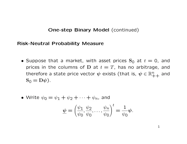
One-step Binary Model (continued) Risk-Neutral Probability Measure • Suppose that a market, with asset prices S 0 at t = 0, and prices in the columns of D at t = T , has no arbitrage, and therefore a state price vector ψ exists (that is, ψ ∈ R n ++ and S 0 = D ψ ). • Write ψ 0 = ψ 1 + ψ 2 + · · · + ψ n , and � t � = 1 ψ 1 , ψ 2 , . . . , ψ n ψ = ψ . ψ 0 ψ 0 ψ 0 ψ 0 1
• The entries of ψ are strictly positive and sum to 1, and may therefore be interpreted as probabilities associated with the various market states at t = T . • The equation S 0 = D ψ can be rewritten S 0 = ψ 0 D ψ = ψ 0 E [ S T ] , where E [ · ] represents expectation with respect to this set of probabilities, and S T is the random vector of asset prices at t = T . 2
• We interpret ψ 0 as a discount factor , and state this as the price of an asset at t = 0 is its expected payoff at t = T , discounted to present value. • But note that these probabilities are derived from a set of weights in a convexity argument, and not from a “view” about the likely state of the market at t = T . 3
• Risk-free borrowing: suppose that there is a portfolio θ whose value is 1 in all states of the market; that is, D t θ = 1 . • The price of this portfolio at t = 0 is then ψ 0 ; zero-coupon Treasury securities play this rˆ ole, and their prices are used to define the risk-free discount factors. • So if there is such a portfolio, the discount factor ψ 0 is unique, even if the state price vector is not. • The discount factor defines the risk-free interest rate through ψ 0 = e − rT . 4
• Attainable claim: a claim C (defined by a vector of payoffs C = ( C 1 , C 2 , . . . , C n ) t ∈ R n ) is attainable if it is replicated by some portfolio. – That is, C = D t φ for some φ ∈ R N . • In a market with no arbitrage and with riskless borrowing, the price at t = 0 of an attainable claim C is ψ 0 E Q [ C ], where E Q [ · ] denotes expected value with respect to a measure Q derived from some state price vector. • Note that we did not need to construct the replicating port- folio to price C , only an appropriate Q . 5
• Risk-neutral probabilities: every Q derived from some state price vector is called a risk-neutral probability measure or an equivalent martingale measure . • A risk-neutral investor is one who prices any asset at its discounted expected value, so a risk-neutral investor who believed that Q describes the true uncertainty in the market would use these prices. • Of course, no such investor exists, so no risk-neutral Q really represents the true market uncertainty. 6
• Complete market: a market is complete if every possible contingent claim C is attainable. – That is, for every C ∈ R n , we can find a portfolio φ with C = D t φ . – In other words, the column space of D t is R n . • Hence our market is complete if and only if D is of full rank n . – This requires that N ≥ n : at least as many assets as states of the market. 7
• In an arbitrage-free market, D is of full rank n if and only if the state price vector ψ , and hence the risk-neutral measure Q , is unique: – If D is of full rank n , and ψ and ψ ′ are two state price vectors, then S 0 = D ψ = D ψ ′ , so D ( ψ − ψ ′ ) = 0 , and because D is of full rank, ψ − ψ ′ = 0 . – Conversely, if D is not of full rank, D δ = 0 for some δ � = 0 . If ψ is a state price vector, then for small enough ǫ , ψ + ǫ δ � = ψ is also a state price vector. 8
Summary of Single Period Model • The market is arbitrage-free if and only if there exists a mar- tingale measure Q . • An arbitrage-free market is complete if and only if Q is unique. • The no-arbitrage price of an attainable claim C is e − rT E Q [ C ]. 9
Recommend
More recommend
Explore More Topics
Stay informed with curated content and fresh updates.
