COMP331/557 Chapter 6: Optimisation in Finance: Cash-Flow - PowerPoint PPT Presentation
COMP331/557 Chapter 6: Optimisation in Finance: Cash-Flow (Cornuejols & Ttnc, Chapter 3) 159 Cash-Flow Management Problem A company has the following net cash flow requirements (in 1000s of ): Month Jan Feb Mar Apr May
COMP331/557 Chapter 6: Optimisation in Finance: Cash-Flow (Cornuejols & Tütüncü, Chapter 3) 159
Cash-Flow Management Problem A company has the following net cash flow requirements (in 1000’s of £): Month Jan Feb Mar Apr May Jun Net cash flow − 150 − 100 200 − 200 50 300 E.g.: In January we have to pay £150k and in March we get £200k. Initially we have no cash but the following possibilities to borrow/invest money: i a line of credit of up to £100k at an interest rate of 1% per month; ii in any one of the first three months, it can issue 90-day commercial paper bearing a total interest of 2% for the three-month period; iii excess funds can be invested at an interest rate of 0.3% per month. Task: We want to maximise the companies wealth in June, while fulfilling all payments. 160
Cash-Flow Management Problem – Modelling as LP Decision Variables ◮ v .. wealth in June ◮ x i .. amount drawn from credit line in month i ◮ y i .. amount of commercial paper issued in month i ◮ z i .. excess funds in month i LP formulation: max v s.t. + − = 150 x 1 y 1 z 1 x 2 + y 2 − 1 . 01 x 1 + 1 . 003 z 1 − z 2 = 100 + − 1 . 01 x 2 + 1 . 003 z 2 − = − 200 x 3 y 3 z 3 x 4 − 1 . 02 y 1 − 1 . 01 x 3 + 1 . 003 z 3 − z 4 = 200 − 1 . 02 y 2 − 1 . 01 x 4 + 1 . 003 z 4 − = − 50 x 5 z 5 − 1 . 02 y 3 − 1 . 01 x 5 + 1 . 003 z 5 − v = − 300 100 x i ≤ ∀ i x i , y i , z i ≥ 0 ∀ i 161
Cash-Flow Management Problem – Modelling as LP cashflow.lp Maximize wealth: v Subject To Jan: x1 + y1 - z1 = 150 Feb: x2 + y2 - 1.01 x1 + 1.003 z1 - z2 = 100 Mar: x3 + y3 - 1.01 x2 + 1.003 z2 - z3 = -200 Apr: x4 - 1.02 y1 - 1.01 x3 + 1.003 z3 - z4 = 200 May: x5 - 1.02 y2 - 1.01 x4 + 1.003 z4 - z5 = -50 Jun: - 1.02 y3 - 1.01 x5 + 1.003 z5 - v = -300 Bounds 0 <= x1 <= 100 0 <= x2 <= 100 0 <= x3 <= 100 0 <= x4 <= 100 0 <= x5 <= 100 -Inf <= v <= Inf End 162
Cash-Flow Management Problem – Modelling as LP Optimal Investment Strategy: Jan: Issue commercial paper for £150k. Gurobi Output Feb: Issue commercial paper for £100k. Solved in 5 iterations and 0.00 seconds Optimal objective 9.249694915e+01 Mar: Issue paper for ≈ £152k and invest ≈ v 92.4969491525 £352k. x1 0.0 y1 150.0 Apr: Take excess to pay outgoing cashflow. z1 0.0 x2 0.0 May: Take a credit of £52k y2 100.0 z2 0.0 Jun: wealth ≈ £92k x3 0.0 y3 151.944167498 z3 351.944167498 x4 0.0 z4 0.0 x5 52.0 z5 0.0 Obj: 92.4969491525 163
The Fundamental Theorem of Asset Pricing (Cornuejols & Tütüncü, Chapter 4) 164
Derivative Securities Derivative Securities ◮ also known as contingent claims ◮ price depend on the value of another underlying security ◮ e.g. European call options European call option Gives the holder the right to buy (or sell, “put option”) ◮ prescribed underlying security ◮ at expiration date (also known as maturity date) ◮ for prescribed amount (called strike price). 165
Example ◮ Share of XYZ stock currently priced at $40. ◮ A month from today, we expect the share price to either double or halve with equal probability. ◮ Consider a European call option on XYZ with strike price $50, which will expire in a month. ◮ Assume that interest rates for cash (borrowing or lending) are zero. ◮ What would be a fair price for the option? European call option payoff function (80 − 50) + = 30 80 = S 1 ( u ) 70 S 0 = $40 ✟✟✟ ✯ and C 0 = ? ✟✟✟ ✯ 60 ❍❍❍ ❍❍❍ (20 − 50) + = 0 50 ❥ 20 = S 1 ( d ) ❥ Payoff from option struck at 50 40 In Section 1.3.2 we obtained a fair price of $10 for the option using a replica- 30 ◮ identical future payoff ⇒ same value today 20 10 ◮ 0 − 10 − 10 10 30 50 70 90 110 120 Share price of XYZ 166 .�����2565�7����9CC������ �2�3�:586 ��8����6 �1�:�6�B:C���7�/:�6������/:3�2����������0�C������2C�����������BD3�6�C�C��C96��2�3�:586����6�C6��B��7�DB6� 2�2:�23�6�2C�9CC������ �2�3�:586 ��8����6�C6��B �9CC����5� 5�: ��8��� ������,0������������� ��� .�����2565�7����9CC������ �2�3�:586 ��8����6 �1�:�6�B:C���7�/:�6������/:3�2����������0�C������2C�����������BD3�6�C�C��C96��2�3�:586����6�C6��B��7�DB6� 2�2:�23�6�2C�9CC������ �2�3�:586 ��8����6�C6��B �9CC����5� 5�: ��8��� ������,0������������� ���
Arbitrage Definition Arbitrage is a trading strategy that: i has positive initial cash flow and no risk of loss later (type A) ii requires no initial cash input, has no risk of loss and has positive probability of making profit in the future (type B) In the example: any price other than $10 for the option would lead to a type A arbitrage. Notes: ◮ Prices adjust quickly so that arbitrage opportunities cannot persist in the marked. ◮ ⇒ Pricing arguments usually assume no arbitrage. 167
Replication (in slightly more general setting) ◮ Consider portfolio of ∆ shares of underlying security and B cash. ◮ Two possible outcomes: ◮ Up-state: ∆ · S 0 · u + B · R , where R = 1 + (risk-less interest rate) ◮ Down-state: ∆ · S 0 · d + B · R ◮ For what values of ∆ and B does the portfolio have the same payoffs C u 1 and C d 1 as the call option? ∆ · S 0 · u + B · R = C u 1 ∆ · S 0 · d + B · R = C d 1 ◮ Solving for ∆ and B gives ∆ = C u 1 − C d B = uC d 1 − dC u 1 1 and S 0 ( u − d ) R ( u − d ) 168
Replication (in slightly more general setting) ◮ Since portfolio is worth S 0 ∆ + B today, this should also be the price for the derivative security, i.e: C 0 = C u 1 − C d + uC d 1 − dC u 1 1 u − d R ( u − d ) = 1 � R − d � 1 + u − R u − d C u u − d C d 1 R ◮ no arbitrage ⇒ d < R < u Definition: Risk-neutral probabilities p u = R − d p d = u − R and u − d u − d Remark: If price � = C 0 then there is arbitrage opportunity. 169
Generalisation of binomial (2-stage) setting ◮ Let ω 1 , . . . , ω m be a finite set of possible states. ◮ For securities S i , i = 0 , . . . n : ◮ S i .. current price (at time 0) 0 ◮ S i 1 ( ω j ) .. future price (at time 1) if in state ω j ◮ S 0 .. risk-less security, i.e. S 0 0 = 1 and S 0 1 ( ω j ) = R ≥ 1 for all j Risk-neutral probabilities A risk-neutral probability measure (RNPM) on the set Ω = { ω 1 , . . . , ω m } is a vector of positive numbers p 1 , . . . , p m such that � m j = 1 p j = 1 and for every security S i , i = 0 , . . . n , m 0 = 1 � S i p j S i . 1 ( ω j ) R j = 1 170
First Fundamental Theorem of Asset Pricing Theorem 6.1 (First Fundamental Theorem of Asset Pricing). A risk-neutral probability measure exists if and only if there is no arbitrage. ◮ Proof is a simple exercise in LP duality. ◮ We will make use of the following result of Goldman and Tucker on the existence of strictly complementary optimal solutions: Theorem 6.2 (Goldman-Tucker Theorem). Consider the following primal-dual pair: min c T x max b T p s.t. A T p = c s.t. Ax ≥ b p ≥ 0 If both, the primal and the dual LP, admit a feasible solution, then there are primal and dual optimal solutions x ∗ , p ∗ such that p ∗ + ( Ax ∗ − b ) > 0 . 171
Arbitrage Detection Using Linear Programming Scenario: ◮ Portfolio ( x 1 , . . . x n ) of European call options S 1 , . . . , S n of same underlying security S . European call option payoff function ◮ Payoff of portfolio: Ψ x ( S 1 ) := � n 70 i = 1 Ψ i ( S 1 ) x i , where 60 ◮ Ψ i ( S 1 ) = ( S 1 − K i ) + , and 50 Payoff from option struck at 50 40 ◮ K i is strike price of call option S i . 30 20 ◮ cost of forming portfolio at time 0 is: � n i = 1 S i 0 x i . 10 0 − 10 − 10 10 30 50 70 90 110 120 Share price of XYZ Determine arbitrage possibility ◮ Negative cost of portfolio with non-negative payoff (type A). ◮ Zero cost and strictly positive payoff (type B). 172 .�����2565�7����9CC������ �2�3�:586 ��8����6 �1�:�6�B:C���7�/:�6������/:3�2����������0�C������2C�����������BD3�6�C�C��C96��2�3�:586����6�C6��B��7�DB6� 2�2:�23�6�2C�9CC������ �2�3�:586 ��8����6�C6��B �9CC����5� 5�: ��8��� ������,0������������� ���
Detecting arbitrage Checking for non-negative payoff: ◮ each Ψ i is piecewise-linear in S 1 with single breakpoint K i ◮ thus Ψ x is piecewise-linear in S 1 with breakpoints K 1 , . . . , K n (assume K 1 ≤ . . . ≤ K n ) ◮ Ψ x is non-negative in [ 0 , ∞ ) , if and only if Ψ x is ◮ non-negative at 0, ◮ non-negative at all breakpoints, and ◮ right-derivative after last breakpoint K n is non-negative. Formally: Ψ x ( 0 ) ≥ 0 Ψ x ( K j ) ≥ 0 , ∀ j , and Ψ x ( K n + 1 ) − Ψ x ( K n ) ≥ 0 . 173
Recommend
More recommend
Explore More Topics
Stay informed with curated content and fresh updates.












![S 0 = D can be rewritten S 0 = 0 D = 0 E [ S T ] , where E [ ] represents](https://c.sambuz.com/944461/s-0-d-s.webp)
