PORTFOLIO CHOICE One Riskless, One Risky Asset Safe asset: gross - PDF document

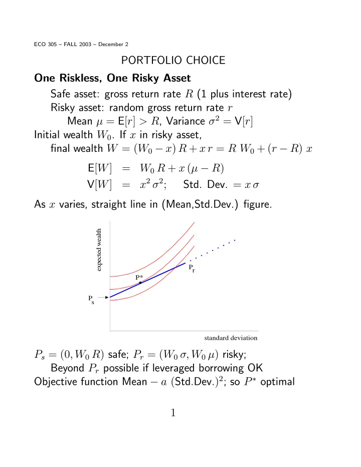
ECO 305 — FALL 2003 — December 2 PORTFOLIO CHOICE One Riskless, One Risky Asset Safe asset: gross return rate R (1 plus interest rate) Risky asset: random gross return rate r Mean µ = E [ r ] > R , Variance σ 2 = V [ r ] Initial wealth W 0 . If x in risky asset, fi nal wealth W = ( W 0 − x ) R + x r = R W 0 + ( r − R ) x E [ W ] = W 0 R + x ( µ − R ) x 2 σ 2 ; V [ W ] = Std. Dev. = x σ As x varies, straight line in (Mean,Std.Dev.) fi gure. expected wealth P r P* P s standard deviation P s = (0 , W 0 R ) safe; P r = ( W 0 σ , W 0 µ ) risky; Beyond P r possible if leveraged borrowing OK Objective function Mean − a ( Std.Dev. ) 2 ; so P ∗ optimal 1

Two Risky Assets W 0 = 1 ; Random gross return rates r 1 , r 2 Means µ 1 > µ 2 ; Std. Devs. σ 1 , σ 2 , Correl. Coe ff t. ρ Portfolio ( x, 1 − x ) . Final W = x r 1 + (1 − x ) r 2 E [ W ] = x µ 1 + (1 − x ) µ 2 = µ 2 + x ( µ 1 − µ 2 ) V [ W ] = x 2 ( σ 1 ) 2 + (1 − x ) 2 ( σ 2 ) 2 + 2 x (1 − x ) ρ σ 1 σ 2 = ( σ 2 ) 2 − 2 x σ 2 ( σ 2 − ρ σ 1 ) + x 2 [( σ 1 ) 2 − 2 ρ σ 1 σ 2 + ( σ 2 ) 2 ] expected wealth P* P 1 P m P 2 standard deviation Diversi fi cation can reduce variance if ρ < min [ σ 1 / σ 2 , σ 2 / σ 1 ] P 1 , P 2 points for the two individual assets P m minimum-variance portfolio Portion P 2 P m dominated; P m P 1 e ffi cient frontier Continuation past P 1 if short sales of 2 OK Optimum P ∗ when preferences as shown 2

One Riskless, Two Risky Assets First combine two riskies; then mix with riskless expected wealth P 1 P P* F P r P Ph P m s P 2 standard deviation This gets all points like P h on all lines like P s P r E ffi cient frontier P s P F tangential to risky combination curve Then along curve segment P F P 1 if no leveraged borrowing; continue straight line P s P F if leveraged borrowing OK With preferences as shown, optimum P ∗ mixes safe asset with particular risky combination P F “Mutual fund” P F is the same for all investors regardless of risk-aversion (so long as optimum in P s P F ) Even less risk-averse people may go beyond P F including corner solution at P 1 or tangency past P 1 if can sell 2 short to buy more 1 3

CAPITAL ASSET PRICING MODEL Individual investors take the rates of return as given but these must be determined in equilibrium Add supply side — fi rms issue equities Take production, pro fi t-max as exogenous Two fi rms, pro fi ts Π 1 and Π 2 . Means E [ Π 1 ] , E [ Π 2 ] ; Variances V [ Π 1 ] , V [ Π 2 ] ; Covariance Cov [ Π 1 , Π 2 ] Safe asset (government bond) sure gross return rate R Market values of fi rms F 1 , F 2 ; to be solved for (endogenous) (Random) rates of return r 1 = Π 1 /F 1 and r 2 = Π 2 /F 2 , and for whole market, r m = ( Π 1 + Π 2 ) / ( F 1 + F 2 ) After a lot of algebra, important results: E [ r 1 ] − R = Cov [ r 1 , r m ] (1) { E [ r m ] − R } V [ r m ] Risk premium on fi rm-1 stock depends on its systematic risk (correlation with whole market) only, not idiosyncratic risk (part uncorrelated with market) Coe ffi cient is beta of fi rm-1 stock F 1 = E [ Π 1 ] − A Cov [ Π 1 , Π 1 + Π 2 ] (2) R where A is the market’s aggregate risk-aversion (usually small) Value of fi rm = present value of its pro fi ts adjusted for systematic risk, and discounted at riskless rate of interest 4

ROCKET-SCIENCE FINANCE Equity, debt etc - complex pattern of payo ff s in di ff erent scenarios: vector S = ( S 1 , S 2 , . . . ) Owning security S is full equivalent to owning portfolio of Arrow-Debreu securities (ADS): S 1 of ADS 1 , S 2 of ADS 2 , . . . In equilibrium, no “riskless arbitrage” pro fi t available So relation bet. price P S of S and ADS prices p i : P S = S 1 p 1 + S 2 p 2 + . . . Converse example: Two scenarios, two fi rms’s shares payo ff MicTel ( M 1 , M 2 ) , BioWiz ( B 1 , B 2 ) . If X M of MicTel + X B of BioWiz ≡ 1 of ADS 1 , X M M 1 + X B B 1 = 1 , X M M 2 + X B B 2 = 0 B 2 − M 2 X M = , X B = M 1 B 2 − B 1 M 2 M 1 B 2 − B 1 M 2 One of these may be negative: need short sales 5

ADS’s can be “constructed” from available securities Then no-arbitrage-in-equilibrium condition: P 1 = X M P MicTel + X B P BioWiz Similarly P 2 . So the “constructed” ADS’s can be priced. Every fi nancial asset is de fi ned by its vector of payo ff s in all scenarios. Therefore it can be priced using these prices of all ADS’s (“pricing kernel”) Examples — options and other derivatives General idea: Markets for risks are complete, and achieve Pareto-e ffi cient allocation of risks if enough securities exist that their payo ff vectors span the space of wealths in all scenarios “Rocket-science fi nance” extends this idea to in fi nite-dimensional spaces of scenarios If sequence of periods, need enough markets to span the scenarios one-period ahead, and then rebalance portfolio by trade (dynamic hedging) Finance = General equilibrium + Linear algebra ! Recent research: (1) Asset pricing with incomplete markets (2) Strategic trading with / against asymmetric info 6