Bigger Models General stock model The market consists of a riskless - PowerPoint PPT Presentation

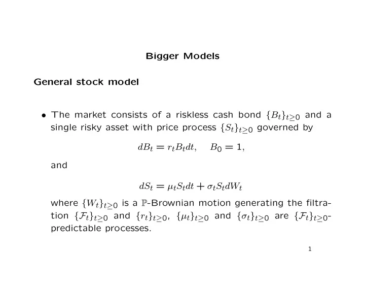
Bigger Models General stock model • The market consists of a riskless cash bond { B t } t ≥ 0 and a single risky asset with price process { S t } t ≥ 0 governed by dB t = r t B t dt, B 0 = 1 , and dS t = µ t S t dt + σ t S t dW t where { W t } t ≥ 0 is a P -Brownian motion generating the filtra- tion {F t } t ≥ 0 and { r t } t ≥ 0 , { µ t } t ≥ 0 and { σ t } t ≥ 0 are {F t } t ≥ 0 - predictable processes. 1

• The real meaning of these SDEs is �� t � B t = exp 0 r s ds , and �� t � t µ s − 1 � � � 2 σ 2 S t = S 0 exp ds + 0 σ s dW s . t 0 • For these integrals to be well defined, we must assume that � t � t � t 0 σ 2 0 | r s | ds, 0 | µ s | ds, and s ds are all finite with P -probability 1. 2

The risk-neutral measure • The discounted stock price S t = B − 1 ˜ S t t satisfies d ˜ S t = ( µ t − r t )˜ S t dt + σ t ˜ S t dW t . • If { ˜ W t } t ≥ 0 is defined by W t = dW t + µ t − r t d ˜ dt, σ t then d ˜ S t = σ t ˜ S t d ˜ W t . 3

• By Girsanov’s theorem, if Q is defined by � t � t 0 γ s dW s − 1 d Q � � � 0 γ 2 � = exp − s ds � 2 d P � F t with γ t = µ t − r t , σ t � � then { ˜ W t } t ≥ 0 is Q -Brownian motion and { ˜ S t } t ≥ 0 is a - Q , {F t } t ≥ 0 martingale. • So Q is the risk-neutral (equivalent martingale) measure. 4

• More restrictions: – For Girsanov’s theorem to apply, we need � t 1 � � 2 γ 2 E P exp < ∞ ; s ds 0 � � – To ensure that { ˜ S t } t ≥ 0 is a Q , {F t } t ≥ 0 -martingale, and not just a local martingale, we need Novikov’s condition: � t 1 � � 2 σ 2 E Q exp < ∞ . s ds 0 5

Replicating a claim � � • If C T is F T -measurable, define the Q , {F t } t ≥ 0 -martingale { M t } t ≥ 0 by B − 1 � M t = E Q � � � F t T C T . � • By the martingale representation theorem, there exists a pre- dictable process { θ t } t ≥ 0 such that � t 0 θ s d ˜ M t − M 0 = W s � t 0 φ s d ˜ = S s where θ t φ t = . σ t ˜ S t 6

• If ψ t = M t − φ t ˜ S t , the portfolio ( ψ, φ ) is self-financing with value at time t V t = φ t S t + ψ t B t = B t M t and in particular V T = B T M T = C T . • So the self-financing portfolio ( ψ, φ ) replicates the claim. 7

Generalized Feynman-Kac • Special case: r t and σ t (but not necessarily µ t ) depend on only t and S t . • Then V t = F ( t, S t ) , where F satisfies 2 σ ( t, x ) 2 x 2 ∂ 2 F ∂t ( t, x )+1 ∂F ∂x 2 ( t, x )+ r ( t, x ) x∂F ∂x ( t, x ) − r ( t, x ) F ( t, x ) = 0 . 8

• In the yet more special case where r t and σ t are functions of only t , and C T = f ( S T ) is a European claim, the value is the same as in the constant r and σ case, with: – r replaced by the average � T 1 ¯ r = r ( s ) ds ; T − t t – σ 2 replaced by the average � T 1 σ 2 = σ ( s ) 2 ds. ¯ T − t t 9