Martingales in Finance F. Ortu (Bocconi U. & IGIER) Workshop on - PowerPoint PPT Presentation
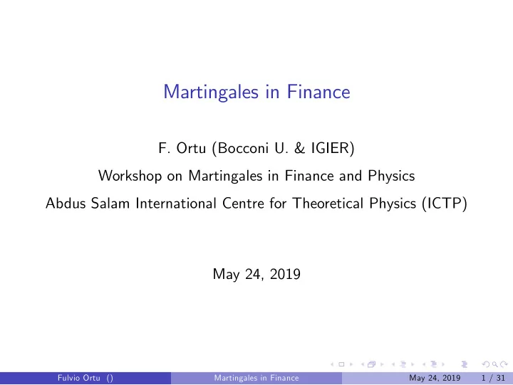
Martingales in Finance F. Ortu (Bocconi U. & IGIER) Workshop on Martingales in Finance and Physics Abdus Salam International Centre for Theoretical Physics (ICTP) May 24, 2019 Fulvio Ortu () Martingales in Finance May 24, 2019 1 / 31
Martingales in Finance F. Ortu (Bocconi U. & IGIER) Workshop on Martingales in Finance and Physics Abdus Salam International Centre for Theoretical Physics (ICTP) May 24, 2019 Fulvio Ortu () Martingales in Finance May 24, 2019 1 / 31
Why Martingales in Finance? E¢cient Markets Hypothesis (EMH): prices in …nancial markets should incorporate all available information Crucial for EMH: the prices at which …nancial securities trade must not allow for arbitrage opportunities I it must not be possible to trade in such a way that you never “lose” and you “win” with positive probability Fundamental Theorem of Finance (FTF): no arbitrage holds if and only if “suitably normalized” securities prices are martingales under a “suitable” probability The “suitable” probability in the FTF takes the name of Risk-Neutral Probability/Equivalent Martingale measure I it is di¤erent from the physical probability, i.e. the probability that governs the actual law of motion of prices Fulvio Ortu () Martingales in Finance May 24, 2019 2 / 31
To be on the same page..... T � < a set of time-indexes � � Ω , F , P , fF t g t 2T a …ltered probability space f X ( t ) g t 2T a Stochastic Process i.e. I X ( t ) F t � measurable (plus some integrability condition....) E [ � / F t ] the conditional expectation operator De…nition f X ( t ) g t 2T is a martingale if � � F t � X ( t ) = E X ( s ) 8 s , t 2 T , s � t , Fulvio Ortu () Martingales in Finance May 24, 2019 3 / 31
Plan of the Talk A very simple one-period model to grasp the basic intuition Expanding on the simple model: the discrete-time case The continuous-time model of Black and Scholes The general continuous-time cases: a primer Fulvio Ortu () Martingales in Finance May 24, 2019 4 / 31
A simple one-period model Dates: t = 0 , 1 (today, tomorrow) States: Ω = f ω 1 , ��� , ω K g , Probabilities: P ( ω k ) > 0 N risky investments (e.g. shares of a risky business) plus 1 riskless investment (e.g. money in the bank) I S j ( 0 ) share price today of risky investment j I S j ( 1 ) ( ω k ) share value tomorrow of risky investment j in state k I r = interest rate: 1 $ in the bank at time 0 becomes ( 1 + r ) $ at time 1 Fulvio Ortu () Martingales in Finance May 24, 2019 5 / 31
Investment strategies and trading ϑ 1 , . . . , ϑ N units held of N risky investments ϑ 0 money in the bank today Total money invested today N ∑ V ϑ ( 0 ) = ϑ 0 + ϑ j S j ( 0 ) j = 1 Total value generated tomorrow in state k N ∑ V ϑ ( 1 ) ( ω k ) = ϑ 0 ( 1 + r ) + ϑ j S j ( 1 ) ( ω k ) j = 1 Fulvio Ortu () Martingales in Finance May 24, 2019 6 / 31
Arbitrage De…nition (Arbitrage Opportunity) An investment strategy ϑ such that V ϑ ( 0 ) � 0 , V ϑ ( 1 ) ( ω k ) � 0, for all k and for some ¯ V ϑ ( 1 ) ( ω ¯ k ) > 0, k In words: an investment strategy whose cost today is non positive, whose revenue tomorrow is non-negative, and the revenue tomorrow is positive in at least one state (i.e. with positive probability) When arbitrages exist markets unravel Fulvio Ortu () Martingales in Finance May 24, 2019 7 / 31
The Fundamental Theorem of Finance (FTF) Theorem The following are equivalent: no-arbitrage holds; 1 there exists Q ( ω k ) > 0 for all k such that for all j 2 1 + r E Q [ S j ( 1 )] 1 S j ( 0 ) = , 1 + r ∑ K 1 k = 1 Q ( ω k ) S j ( 1 ) ( ω k ) In words: arbitrage opportunities disappear if and only if there is some probability Q that makes the price today of each security equal to the discounted expected value tomorrow Where are the martingales? Fulvio Ortu () Martingales in Finance May 24, 2019 8 / 31
Martingales and Finance, act 1 S j ( 0 ) , S j ( 0 ) while De…ne the Discounted Price as follows: e 1 S j ( 1 )( ω k ) , e 1 + r S j ( 1 ) ( ω k ) , k = 1 , ..., K Statement 2 in the FTF becomes then S j ( 0 ) = E Q h i e e S j ( 1 ) a (Mickey Mouse......) martingale! The jargon for Q : I Risk-Neutral probability in Finance: only averages matter, variance/risk is irrelevant I Equivalent Martingale Measure in Math: Q and the physical probability P are equivalent measures (but Q 6 = P in general!!) Fulvio Ortu () Martingales in Finance May 24, 2019 9 / 31
The multi-period framework Dates: t = 0 , 1 , ....., T � � Ω , F , P , fF t g T A …ltered probability space t = 0 S j ( t ) the price at time t of risky investment j I S j ( t ) an F t � measurable , square � integrable random variable I 1 in the bank at time 0 becomes ( 1 + r ) t at time t Discounted prices 1 e S j ( t ) , 1 + r S j ( t ) , t = 0 , 1 , ..., T Fulvio Ortu () Martingales in Finance May 24, 2019 10 / 31
Equivalent Martingale Measures (EMMs) De…nition An Equivalent Martingale Measure (EMM) is a probability measure Q v P such that L = dQ 1 + r 2 L 2 L i ) dP > 0, n o T e ii ) S j ( t ) t = 0 is a Q� martingale 8 j that is S j ( t ) = E Q h . i e e S j ( s ) F t , 8 s � t EMMs extend the notion seen in the very simple one-period case: for t = 0 , s = 1 S j ( 0 ) = E Q h . i = E Q h i e e e S j ( 1 ) F 0 S j ( 1 ) Fulvio Ortu () Martingales in Finance May 24, 2019 11 / 31
The multi-period FTF Theorem The following are equivalent in a multiperiod market: (a suitably extended notion of) no-arbitrage holds 1 there exist EMMs 2 How many EMMs? I One and only one if and only if markets are complete! What’s their use (besides characterizing No-Arbitrage)? I To price new securities (stocks, bonds, options, other derivative securities....) constantly added to the market by the …nance industry. More on this later Fulvio Ortu () Martingales in Finance May 24, 2019 12 / 31
The Continuous-time Black-Scholes (BS) Model: the primitives Dates: t 2 [ 0 , T ] A Standard Brownian Motion f W t g t 2 [ 0 , T ] � � � F W � Ω , F , P , A …ltered probability space t t 2 [ 0 , T ] n o F W I t 2 [ 0 , T ] the …ltration generated by f W t g t 2 [ 0 , T ] t Only two investment opportunities: a share of common stock and a bank account Fulvio Ortu () Martingales in Finance May 24, 2019 13 / 31
The stock and the bank account The stock price S ( t ) follows a Geometric Brownian Motion under the physical probability P S ( t ) = S ( 0 ) e ( µ � 1 2 σ 2 ) t + σ W ( t ) Ito’s Lemma yields dS ( t ) = µ S ( t ) dt + σ S ( t ) dW ( t ) Letting δ = ln ( 1 + r ) , 1 Euro in the bank at time 0 becomes B ( t ) = ( 1 + r ) t � e δ t , i.e. dB ( t ) = δ B ( t ) dt Discounted stock price: e S ( t ) = e � δ t S ( t ) , so that d e S ( t ) = ( µ � δ ) e S ( t ) dt + σ e S ( t ) dW ( t ) Fulvio Ortu () Martingales in Finance May 24, 2019 14 / 31
Economic interpretation and properties The stock has a lognormal distribution: I therefore stock price never falls below zero, satisfying the economic condition of limited liability Basic economic assumption: µ > δ I the average instantaneous return on the stock µ is greater than the instantaneous return δ from keeping money in the bank I µ � δ > is called the risk premium: compensation to stockholders for the risk from holding stocks Both S ( t ) and e S ( t ) display a drift: I neither one is a martingale! Where are the martingales in the BS model? Fulvio Ortu () Martingales in Finance May 24, 2019 15 / 31
The EMM in the BS model: existence Theorem (Girsanov) Under suitable integrability conditions on ν ( t ) there exists a probability Q � P s.t. dW Q ( t ) = ν ( t ) dt + dW ( t ) is a Standard Brownian Motion Therefore, in the BS model there exists Q � P s.t. 2 3 6 7 ( µ � δ ) 6 7 d e = σ e S ( t ) S ( t ) 6 dt + dW ( t ) 7 4 σ 5 | {z } ν ( t ) = σ e S ( t ) dW Q ( t ) i.e. there exists Q � P such that e S ( t ) under Q is a driftless di¤usion: a Martingale! Fulvio Ortu () Martingales in Finance May 24, 2019 16 / 31
The EMM in the BS model: properties By Ito’s Lemma 2 σ 2 t + σ W Q ( t ) S ( t ) = S ( 0 ) e � 1 e Therefore, since E Q h i e S ( t ) = S ( 0 ) and S ( t ) = e δ t e S ( t ) , then E Q [ S ( t )] = e δ t S ( 0 ) Under Q the average instantaneous return on the stock is δ , the same as the bank account: I the notion of Risk-Neutral Probability! Fulvio Ortu () Martingales in Finance May 24, 2019 17 / 31
Trading in the BS model ϑ 0 ( t ) , ϑ 1 ( t ) I money in the bank, stock shares held at time t V ϑ ( t ) value invested at time t : V ϑ ( t ) = ϑ 0 ( t ) B ( t ) + ϑ 1 ( t ) S ( t ) De…nition (Self-…nancing trading) A trading strategy is self-…nancing if dV ϑ ( t ) = ϑ 0 ( t ) dB ( t ) + ϑ 1 ( t ) dS ( t ) equivalently if the discounted value e V ϑ ( t ) = e � δ t V ϑ ( t ) satis…es d e V ϑ ( t ) = ϑ 1 ( t ) d e S ( t ) Fulvio Ortu () Martingales in Finance May 24, 2019 18 / 31
Self-…nancing trading and arbitrage A self-…nancing trading strategy ϑ 0 ( t ) , ϑ 1 ( t ) is an arbitrage opportunity if V ϑ ( 0 ) � 0 1 V ϑ ( T ) � 0 P - almost surely 2 P [ V ϑ ( T ) > 0 ] > 0 3 The same economic intuition as in the simple one-period case (technicalities aside) Fulvio Ortu () Martingales in Finance May 24, 2019 19 / 31
Recommend
More recommend
Explore More Topics
Stay informed with curated content and fresh updates.
