Ryo Onishi 1 , Keigo Matsuda 1 , Yuichi Kunishma 2 , Dmitry - PowerPoint PPT Presentation

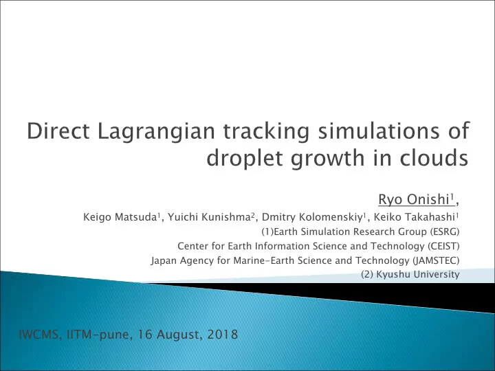
Ryo Onishi 1 , Keigo Matsuda 1 , Yuichi Kunishma 2 , Dmitry Kolomenskiy 1 , Keiko Takahashi 1 (1)Earth Simulation Research Group (ESRG) Center for Earth Information Science and Technology (CEIST) Japan Agency for Marine-Earth Science and Technology (JAMSTEC) (2) Kyushu University IWCMS, IITM-pune, 16 August, 2018

} We choose research themes, in Marine-Earth science, that are interesting in physics and challenging in computation. Our research themes are often related with tu turbule lence . 2

Ø Seamless simulations for global, regional and street scales Ø atmosphere-ocean coupled gl global scale re regional sale st street sc scale O(1~10 km) resolution O(100 m~1km) resolution O(1~10 m) resolution 3 This movie is displayed at the Japan Science Museum (Miraikan) in Tokyo.

Group Mission Research and Modeling of multiscale, multiphase and non-equilibrium turbulence processes in marine and Earth science Apply Development of Multi-scale weather/climate model ： MSSG + IoT + AI Social Implementation Promotion of Marine and Earth informatics

Multiscale, multiphase and non-equilibrium turbulence processes in marine and Earth Science ICL 、 DWD 、 Delaware univ. 、 Nagoya Tech. univ. cloud turbulence and droplet collisional growth Cardiff univ., Osaka univ. collisional breakup cloud turbulence and radar observation This talk convective clouds ＝ turbulent clouds Nagoya Tech. univ., Tokyo univ., Tokyo Sci. univ. turbulent transportation seaspray-enhanced turbulent heat exchange NIMS, CRIEPI Corrosion due to airborne seasalt Kyoto univ. non-equilibrium turbulence in urban&tree canopies mass and heat transfer in wind-wave turbulence Nagoya univ., TITEC, ICL

} Cloud microphysics simulations ◦ Eulerian and Lagrangian frameworks ◦ Droplet growth in clouds } Direct Lagrangian tracking simulations ◦ Turbulent collision kernels ◦ Droplet collision growth in box turbulence ◦ Droplet growth in a vertically-developing cloud } Miscellaneous (on-going work) ◦ Size-resolving simulation ◦ Turbulence influence on Radar reflectivity 6

Eu Euler fr framewo work La Lagrangian fr framewo work Me Method Bu Bulk Bi Bin Di Dire rect Su Super-Dr Droplet Prognosed Moments of size distribution Particle attributions variables ò x p , u p , r p etc… = n n M m f ( m ) dm k k Implicit Explicit Explicit Size distribution Num. of O(10~100) -- ＜１０ Categories Multiplicity -- 1≦ 1 (direct) Illustration References Many Many (incl. Shima et al. (2009) Onishi et al. (2015) QJRMS JAS; Gotoh et al. Onishi & (2016) NJP Takahashi(2012) Lagrangian cloud model JAS) DI DIRECT Lagrangian cloud model 7

} Activation } Condensation/evaporation } Collision (coagulation) → challenging in HPC } Settling(Precipitation) e.g., Shaw (2003) Annu. Rev. Fluid Mech. 8

} Quick rain formation in turbulent clouds (refs: Shaw (2003), Grabowski & Wang (2013), etc…) } Industrial flows e.g., spray combustion, pulverized coal combustion Sun gas dust http://www.colorado.edu/MCEN/cmes planetesimal } Dust growth in protoplanetary disks s (refs: Pan et al. (2011), Okuzumi et al. (2012) etc…) protoplanet s planets http://www-tap.scphys.kyoto-u.ac.jp/hayashi/lectures/kokubo.pdf 9

(1)Onishi et al. (2011) J. Comput. Phys. (2)Onishi et al. (2013) J. Comput. Phys. } Flow (3)Onishi et al. (2015) J. Atmos. Sci. ◦ 4 th -order FDM ◦ 2 nd -order R-K ◦ RCF (1) : large-scale forcing ◦ 3D domain decomposition } Particles ◦ Lagrangian tracking ◦ 2 nd -order R-K ◦ Cell-index method ◦ BiSM (2) for hydrodynamic interaction ◦ 3D domain decomposition Following the so-called hybrid DNS approach (Wang et al. 2005; Ayala et al. 2007)

process 0 process 1 } 1D domain decomposition process 2 } 2D domain decomposition } 3D domain decomposition 2D or 3D dd is required for HPC. 11

} Originally developed for MD simulation. } (1)Divide computational domain is into cells. } (2)Make the list that shows which particle locates in which cell. } (3)Detect pairs in 27 cells * using the cell index. *14 cells are enough for sequential procedure This method can reduce the cost for detecting neighboring pairs: O(Np 2 ) → O(Np) 12

Ø Flow motion: Imcompressible N-S eq. Ø Particle motion: Flow ： Euler method Particle: Lagrangian monodisperse, no-gravity tracking method # of grids k max l η R λ # of particles 64 3 2.0 54.9 32 3 Onishi et al. (2009) PoF 64 3 128 3 2.0 81.3 128 3 256 3 2.0 126 256 3 512 3 2.0 207 ES2 500 3 1,000 3 2.0 323 1000 3(=1 Onishi et al. (2013) JCP, 2,000 3 2.0 527 Onishi & Vassilicos (2014) JFM billion) 4,000 3 2.0 860 1.6 billion K 6,000 3 2.0 1,120 5.4 billion Onishi & Seifert (2016) ACP new ES→ 8,192 3 2.0 1,390 8.2 billion 13

} Collision frequency N c [1/(m 3 s)] ; N c ( r 1 , r 2 )= n p ( r 1 ) n p ( r 2 )K c ( r 1 , r 2 ), where n p [1/m 3 ] is the particle number density. } Gravitational collision kernel = p - 2 K c ( r , r ) R V ( r ) V ( r ) ¥ ¥ 1 2 1 2 1 ( R : collision radius (= r 1 + r 2 ), V ∞ :settling velocity ) π R 2 14

<<spherical formulation (Wang et al., (2000) JFM ) >> ( ) = p = = 2 K r , r 2 R | w ( x R ) | g ( x R ) c 1 2 r R : collision radius (=r 1 +r 2 ) | w r | : radial relative velocity at contact g (R) : radial distribution function at contact (clustering effect) 2 æ ö r τ p : particle relaxation time t 2 r ç ÷ = = p St p τ η : Kolmogorov time t ç ÷ r 9 l è ø h h f St~ 0 St= 0.2 radius[μm] St CCN <1 <<1 clustering Cloud droplets 10 0.01 30 0.1 Rain drops 100 1 St= 4 St= 1 Large drops 1000< 10 Clustering enlarges the collision probability. 15

Fig 2 in Onishi & Seifert (2016) ACP ● Ireland et al. (2016) JFM Lines show predictions based on the “intermittency hypothesis” （ Onishi & Vassilicos 2014 JFM ） ● Re λ =1390 This Re-dependency has been included in a turbulent collision kernel model (Onishi & Seifert 2016, ACP ) and in bulk Decreasing for increasing Re for 1/3<St<1 parameterizations (Seifert & Onishi 2016, ACP ) 16

} Mechanism of the Re-dependence of clustering ◦ Onishi & Vassilicos (2014) JFM } Modeling of turbulent collision kernel ◦ Onishi & Seifert (2016) ACP (where fortran code provided as a suppliment) } Bulk parameterizations of turbulent collision growth (autoconversion and accretion) ◦ Seifert & Onishi (2016) ACP

*Gravitational droplet Settling (precipitation) is considered as well. Onishi et al. (2015) JAS

19

} [For robust reference data] We can directly analyze multi-scale phenomena without separating macro- and micro-scales. ◦ Recirculation of rain drops (Naumann & Seifert 2016 JAMES) or of ice particles (Yang et al. 2015 JGR Atmos.) ◦ Evaporative and radiative cooling in cloud turbulent mixing layer (e.g., de Lozer & Mellado 2013JAS, Kumar et al. 2014JAS) but several physics (particularly, co collisions ) have been skipped in literature } [For intrinsic statistical fluctuations] We can obtain new kind of information regarding statistical fluctuations and can investigate individual realizations, not the ensemble-averaged statistics. NB. [Prediction error]=[Practical error] + [I [Intrinsic error or] 20

Onishi et al. (2015) J. Atmos. Sci. } Fluid and Scalars (Euler method) Onishi et al. (2011) J. Comput. Phys. } Particles (Lagragian tracking method) disturbance vel. due to hydrodynamic interactions. (Onishi et al. (2013) J. Comput. Phys. ) 21

～ Typical Cu 22

～ Typical Cu } Initial size dist. of the group of droplets: where x is the particle mass, x m (set to m ( r =15µm) ) is the mean particle mass. 23

Stochastic Collection Equation (SCE) K coal =E coal *E c *K c ¶ æ ö n ( m ) 1 ¥ m ò ò ç p ÷ = - - - K ( m m ' , m ' ) n ( m m ' ) n ( m ' ) dm ' K ( m , m ' ) n ( m ) n ( m ' ) dm ' ç ÷ ¶ coal p p coal p p t 2 è ø 0 0 col } Coalescence efficiency: E coal =1 } Collision efficiency: ◦ E c =1 for NoHI ◦ E c = E c (Pinsky et al., 2001) for NoT-HI ◦ E c = E c (Pinsky et al., 2001)* η E (Wang et al. 2008) for T-HI } Collision kernel: ◦ K c [NoT]=gravitational kernel ◦ K c [T]=Onishi turbulent kernel (Onishi & Seifert 2016) 24

Onishi et al. (2015) J. Atmos. Sci. ∫ ξ ( φ )d y , where φ =log 10 r, obtains the liquid mixing ratio [kg/m 3 ]. Stagnant (NoT) case With HI Without HI Rain Rain drops drops φ =log 10 r Without HI, droplets grow unrealistically too fast. Proof of the relevant role of HI 25

Onishi et al. (2015) J. Atmos. Sci. ∫ ξ ( φ )d y , where φ =log 10 r, obtains the liquid mixing ratio [kg/m 3 ]. HI case Stagnant (NoT) Turbulence (T) Rain Rain drops drops φ =log 10 r Turbulence promotes size evolutions. Good agreement between SCE and LCS. 26

Liquid water is classified into CLOUD (small droplets, usually smaller than 40um in radius) and RAIN categories. } autoconversion ◦ CLOUD + CLOUD =>RAIN collision/coagulation } accretion ◦ CLOUD + RAIN =>RAIN } condensation ◦ vapor ó CLOUD, RAIN accre ac retion au autoconvers rsion e.g., Shaw (2003) Annu. Rev. Fluid Mech. 27