Rough solutions of the Stochastic Birnir The Navier-Stokes - PowerPoint PPT Presentation
Turbulence Rough solutions of the Stochastic Birnir The Navier-Stokes Equation Stochastic Closure of Navier-Stokes The Kolmogorov- Bjrn Birnir Obukhov-She- Leveque Scaling Center for Complex and Nonlinear Science The variable
Turbulence Rough solutions of the Stochastic Birnir The Navier-Stokes Equation Stochastic Closure of Navier-Stokes The Kolmogorov- Björn Birnir Obukhov-She- Leveque Scaling Center for Complex and Nonlinear Science The variable Department of Mathematics, UC Santa Barbara density wind and tunnel University of Iceland, Reykjavík Fitting the data The Error in RICAM, Linz, December 2016 the Fit Existence of Co-authors, Gregory Bewley, Cornell, Michael Sinhuber, Göttingen, John Rough Solutions Kaminsky and Shahab Karmini, UC Santa Barbara Conclusions
Outline Turbulence Birnir 1 The Stochastic Closure of Navier-Stokes The Stochastic 2 The Kolmogorov-Obukhov-She-Leveque Scaling Closure of Navier-Stokes The The variable density wind tunnel 3 Kolmogorov- Obukhov-She- Leveque Scaling Fitting the data 4 The variable density wind tunnel The Error in the Fit 5 Fitting the data Existence of Rough Solutions 6 The Error in the Fit Existence of 7 Conclusions Rough Solutions Conclusions
Outline Turbulence Birnir 1 The Stochastic Closure of Navier-Stokes The Stochastic 2 The Kolmogorov-Obukhov-She-Leveque Scaling Closure of Navier-Stokes The The variable density wind tunnel 3 Kolmogorov- Obukhov-She- Leveque Scaling Fitting the data 4 The variable density wind tunnel The Error in the Fit 5 Fitting the data Existence of Rough Solutions 6 The Error in the Fit Existence of 7 Conclusions Rough Solutions Conclusions
The Deterministic Navier-Stokes Equations Turbulence A general incompressible fluid flow satisfies the Birnir Navier-Stokes Equation The u t + u · ∇ u = ν ∆ u − ∇ p Stochastic Closure of Navier-Stokes u ( x , 0 ) = u 0 ( x ) The Kolmogorov- with the incompressibility condition Obukhov-She- Leveque Scaling ∇ · u = 0 , The variable density wind Eliminating the pressure using the incompressibility tunnel condition gives Fitting the data ν ∆ u + ∇ ∆ − 1 trace ( ∇ u ) 2 u t + u · ∇ u = The Error in the Fit u ( x , 0 ) = u 0 ( x ) Existence of Rough Solutions The turbulence is quantified by the dimensionless Conclusions Taylor-Reynolds number Re λ = U λ ν
The Reynolds Decomposition Turbulence Birnir The velocity is written as U + u , pressure as P + p The U describes the large scale flow, u describes the small Stochastic Closure of scale turbulence Navier-Stokes The This is the classical Reynolds decomposition (RANS) Kolmogorov- Obukhov-She- Leveque ν ∆ U − ∇ P − ∂ Scaling U t + U · ∇ U = ∂ x j R ij The variable density wind tunnel The last term the eddy viscosity, where R ij = u i u j is the Fitting the data Reynolds stress, describes how the small scale The Error in influence the large ones. the Fit Existence of Closure problem : compute R ij . Rough Solutions Conclusions
A Stochastic Closure Turbulence Birnir Large scale flow The Stochastic ν ∆ U − ∇ P − ∂ Closure of U t + U · ∇ U = ∂ x j R ij Navier-Stokes The Kolmogorov- U ( x , 0 ) = U o ( x ) . Obukhov-She- Leveque Scaling Small scale flow The variable density wind ν ∆ u + ∇ ∆ − 1 trace ( ∇ u ) 2 + Noise tunnel u t + u · ∇ u = Fitting the u ( x , 0 ) = u 0 ( x ) . data The Error in the Fit What is the form of the Noise? It will contain both Existence of additive noise and multiplicative u · noise . Rough Solutions Conclusions
Stochastic Navier-Stokes with Turbulent Noise Turbulence Adding the two types of additive noise and the Birnir multiplicative noise we get the stochastic Navier-Stokes The equations describing fully developed turbulence Stochastic Closure of Navier-Stokes ( U + u ) · ∇ u − u · ∇ U + ∇ ∆ − 1 tr ( ∇ u ) 2 ) dt du = ( ν ∆ u − The Kolmogorov- 1 + ∑ t e k ( x )+ ∑ k db k d k | k | 1 / 3 dt e k ( x ) Obukhov-She- c 2 Leveque Scaling k � = 0 k � = 0 The variable M � density wind R h k ¯ N k ( dt , dz )) ∑ + u ( (1) tunnel k � = 0 Fitting the data u ( x , 0 ) = u 0 ( x ) The Error in the Fit Each Fourier component e k = e 2 π ik · x comes with its Existence of Rough own Brownian motion b k t and deterministic bound Solutions | k | 1 / 3 dt Conclusions
Outline Turbulence Birnir 1 The Stochastic Closure of Navier-Stokes The Stochastic 2 The Kolmogorov-Obukhov-She-Leveque Scaling Closure of Navier-Stokes The The variable density wind tunnel 3 Kolmogorov- Obukhov-She- Leveque Scaling Fitting the data 4 The variable density wind tunnel The Error in the Fit 5 Fitting the data Existence of Rough Solutions 6 The Error in the Fit Existence of 7 Conclusions Rough Solutions Conclusions
The Kolmogorov-Obukhov Theory Turbulence Birnir In 1941 Kolmogorov and Obukhov [7, 6, 9] proposed a statistical theory of turbulence The Stochastic Closure of The structure functions of the velocity differences of a Navier-Stokes turbulent fluid, should scale with the distance (lag The Kolmogorov- variable) l between them, to the power p / 3 Obukhov-She- Leveque Scaling E ( | u ( x , t ) − u ( x + l , t ) | p ) = S p = C p l p / 3 The variable density wind tunnel Fitting the data The Error in the Fit Existence of Rough Solutions A. Kolmogorov A. Obukhov Conclusions
The Kolmogorov-Obukhov Refinded Similarity with She-Leveque Intermittency Corrections Turbulence The Kolmogorov-Obukhov ’41 theory was criticized by Birnir Landau for including universal constants C p and later for not including the influence of the intermittency The Stochastic Closure of In 1962 Kolmogorov and Obukhov [8, 10] proposed a Navier-Stokes refined similarity hypothesis The Kolmogorov- ε p / 3 > l p / 3 = C p l ζ p Obukhov-She- S p = C ′ p < ˜ (2) Leveque Scaling l is the lag and ε a mean energy dissipation rate The variable density wind tunnel The scaling exponents Fitting the data ζ p = p 3 + τ p The Error in the Fit Existence of include the She-Leveque intermittency corrections Rough τ p = − 2 p 9 + 2 ( 1 − ( 2 / 3 ) p / 3 ) and the C p are not universal Solutions Conclusions but depend on the large flow structure
Solution of the Stochastic Navier-Stokes Proof of Kolmogorov-Obukhov refined hypothesis Turbulence We solve (1) using the Feynmann-Kac formula, and Birnir Girsanov’s Theorem The The solution is Stochastic Closure of � t � t e Kt e 0 ∇ Uds e 0 dq M t u 0 Navier-Stokes u = � t The � ( t − s ) � t Kolmogorov- + ∑ 0 e K ( t − s ) e ∇ Udr e s dq M t − s 0 Obukhov-She- Leveque k � = 0 Scaling ( c 1 / 2 db k s + d k | k | 1 / 3 ds ) e k ( x ) × The variable k density wind tunnel K is the operator K = ν ∆+ ∇ ∆ − 1 tr ( ∇ u ∇ ) Fitting the data M t is the Martingale The Error in the Fit � t � t 0 ( U + u )( B s , s ) · dB s − 1 0 | ( U + u )( B s , s ) | 2 ds } M t = e {− 2 Existence of Rough Solutions Using M t as an integrating factor eliminates the inertial Conclusions terms from the equation (1)
The Feynmann-Kac formula The computation of the intermittency corrections Turbulence The Feynmann-Kac formula gives the exponential of a Birnir sum of terms of the form The � t � t � t Stochastic � � s dq k = R ln ( 1 + h k ) N k ( dt , dz ) − R h k m k ( dt , dz ) , Closure of Navier-Stokes 0 0 The Kolmogorov- by a computation similar to the one that produces the Obukhov-She- geometric Lévy process [1, 2], m k the Lévy measure. Leveque Scaling The form of the processes The variable density wind tunnel � t � t R ln ( 1 + h k ) N k ( dt , dz ) − R h k m k ( dt , dz ) � � e 0 0 Fitting the data t ln β + γ ln | k | = | k | γ β N k = e N k t The Error in the Fit was found by She and Leveque [11], for h k = β − 1 Existence of Rough Solutions It was pointed out by She and Waymire [12] and by Conclusions Dubrulle [5] that they are log-Poisson processes.
KOSL Scaling of the Structure Functions, higher order Re λ ∼ 16 , 000 Comparison of Theory and Experiments Turbulence Birnir The Stochastic Closure of Navier-Stokes The Kolmogorov- Obukhov-She- Leveque Scaling The variable density wind tunnel Figure: The exponents of the structure functions as a function of Fitting the data order, theory or Kolmogorov-Obukov-She-Leveque scaling (red), The Error in experiments (disks), dns simulations (circles), from [4], and the Fit experiments (X), from [11]. The Kolomogorov-Obukhov ’41 Existence of Rough scaling is also shown as a blue line for comparion. Solutions Conclusions
KOSL Scaling of the Structure Functions, low order Re λ ∼ 16 , 000 Turbulence Birnir The Stochastic Closure of Navier-Stokes The Kolmogorov- Obukhov-She- Leveque Scaling The variable density wind tunnel Figure: The exponents of the structure functions as a function of Fitting the data order ( − 1 , 2 ] , theory or Kolmogorov-Obukov-She-Leveque scaling The Error in (red), experiments (disks), dns simulations (circles), from [4]. The the Fit Kolmogorov-Obukov ’41 scaling is also shown as a blue line for Existence of Rough comparion. Solutions Conclusions
Recommend
More recommend
Explore More Topics
Stay informed with curated content and fresh updates.
