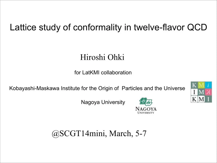
Lattice study of conformality in twelve-flavor QCD Hiroshi Ohki for - PowerPoint PPT Presentation

Lattice study of conformality in twelve-flavor QCD Hiroshi Ohki for LatKMI collaboration Kobayashi-Maskawa Institute for the Origin of Particles and the Universe Nagoya University @SCGT14mini, March, 5-7

LatKMI collaboration K. Hasebe Y. Aoki T. Aoyama M. Kurachi A. Shibata E. Bennett T. Maskawa K. Miura K.I. Nagai E. Rinaldi H. O. T. YAmazaki K .Yamawaki

Introduction

Walking and conformal behavior -> non-perturbative dynamics Many flavor QCD: benchmark test of walking dynamics : Number of flavor α ( µ ): running gauge coupling Asymptotic non-free Conformal window Walking technicolor QCD-like • Understanding of the conformal dynamics is important (e.g. critical phenomena) • Walking technicolor (WTC) could be realized just below conformal window. • What the value of the anomalous dimensions γ ? ( γ : critical exponent ) • Rich hadron structures may be observed in LHC.

LatKMI -Nagoya project (since 2011) Systematic study of flavor dependence in Large Nf QCD using single setup of the lattice simulation Our goals: • Understand the flavor dependence of the theory • Find the conformal window • Find the walking regime and investigate the anomalous dimension ! Status (lattice): T. Yamazaki (poster) Nf=16: likely conformal This talk Nf=12: controversial Nf=8: controversial, our study suggests walking behavior? Nf=4: chiral broken and enhancement of chiral condensate ! M. Kurachi (poster) Observables: talk by K.-i. Nagai (next) pseudoscalar, vector meson -> chiral behavior Glueball (O++) and/or flavor-singlet scalar Is this lighter compared with others? If so, Good candidate of “Higgs” (techni-dilaton). talk by T. Yamazaki E. Rinaldi for gluonic observables (poster)

Our work • use of improved staggered action Highly improved staggered quark action [HISQ] • use MILC version of HISQ action use tree level Symanzik gauge action no (ma) 2 improvement (no interest to heavy quarks)= HISQ/tree Simulation setup • SU(3), Nf=12 flavor simulation parameters two bare gauge couplings ( β ) & four volumes & various fermion masses • β =6/g 2 =3.7, 3.8, and 4.0 • V=L 3 xT: L/T=3/4; L=18, 24, 30, 36 • 0.03 ≦ m f ≦ 0.2 for β =3.7, 0.04 ≦ m f ≦ 0.2 for β =4.0 Statistics ~ 2000 trajectory • Measurement of meson spectrum in particular pseudoscalar (“NG-pion”) mass (M π ), decay constant (F π ) vector meson mass (M ρ ) Machine: φ @ KMI, CX400 @ Kyushu Univ.

N f =12 Result � � � [LatKMI, PRD86 (2012) 054506] and Some updates Preliminary

F π and M π Nf=12 1 0.2 L=18 L=18 L=24 L=24 L=30 L=30 0.8 L=36 L=36 0.15 0.6 M � F � 0.1 0.4 0.05 0.2 0 0 0 0.05 0.1 0.15 0.2 0 0.05 0.1 0.15 0.2 m f m f

Nf=12 theory: Conformal phase v.s. Chiral broken phase From the fermion mass (mf) dependence of the hadron mass, we study the phase structure of the theory. Conformal hypothesis: critical phenomena near the fixed point hyper-scaling, γ : mass anomalous dimension at the fixed point M H � mf 1/(1+ γ ) • F π � mf 1/(1+ γ ) + … (for small mf) • ���� F π /M π → constant (mf → 0) M ρ /M π → constant mf RG flow in mass-deformed conformal field theory(CFT) β β c

Nf=12 theory: Conformal phase v.s. Chiral broken phase From the fermion mass (mf) dependence of the hadron mass, we study the phase structure of the theory. Conformal hypothesis: critical phenomena near the fixed point hyper-scaling, γ : mass anomalous dimension at the fixed point M H � mf 1/(1+ γ ) • F π � mf 1/(1+ γ ) + … (for small mf) • ���� F π /M π → constant (mf → 0) M ρ /M π → constant mf Chiral symmetry breaking hypothesis: π is NG-boson. Chiral perturabation theory (ChPT) works. RG flow in mass-deformed M π 2 � mf (PCAC relation) • conformal field theory(CFT) F π =F+c M π 2 + … (for small mf) • ���� F π /M π → ∞ (mf → 0) β β c

A primary analysis, F π /M π vs M π Nf=12 0.22 0.22 0.22 0.22 0.22 LatKMI L=24 L=18 L=18 L=18 L=18 L=24 L=24 L=24 L=30 L=30 L=30 L=36 0.21 0.21 0.21 0.21 0.21 L=36 β =3.7 F � /M � F � /M � F � /M � F � /M � F � /M � 0.2 0.2 0.2 0.2 0.2 β =4 0.19 0.19 0.19 0.19 0.19 0.18 0.18 0.18 0.18 0.18 0.2 0.4 0.8 1 0.2 0.2 0.2 0.2 0.4 0.4 0.4 0.4 0.6 0.6 0.6 0.6 0.6 0.8 0.8 0.8 0.8 1 1 1 1 M � M � M � M � M � In both of β =3.7 and 4.0, both ratios at L=30 and L=36 seem to be flat in the small mass region, but small volume data (L ≦ 24) shows large finite volume effect. This behavior is contrast to the result in ordinary QCD system

M ρ /M π vs M π Nf=12 1.3 1.3 1.3 1.3 1.3 Flat region L=18 L=18 L=24 L=18 L=18 L=24 L=30 L=24 L=24 L=30 L=36 L=30 1.25 1.25 1.25 1.25 1.25 L=36 β =3.7 M � /M � M � /M � M � /M � M � /M � M � /M � 1.2 1.2 1.2 1.2 1.2 β =4 1.15 1.15 1.15 1.15 1.15 1.1 1.1 1.1 1.1 1.1 0 0 0 0.2 0.2 0.2 0.4 0.4 0.4 0.6 0.6 0.8 0.8 0.8 0 0 0.2 0.2 0.4 0.4 0.6 0.6 0.6 0.8 0.8 M � M � M � M � M � Ratio is almost flat in small mass region (wider than F π /M π ) -> consistent with hyper scaling Volume dependence is smaller than F π /M π . In the large mass region, large mass effects show up. M ρ /M π should be 1, as mf -> infinity.

Conformal hypothesis in infinite volume & finite volume Universal behavior for all hadron masses (hyper-scaling) • Mass dependence is determined by scaling dimension (mass-deformed CFT.) • M H ∝ m 1 / (1+ γ ) F π ∝ m 1 / (1+ γ ) , (infinite'volume'result) f f Our interest : the same low-energy physics with the one obtained in infinite volume limit But all the numerical simulations can be done only in finite size system (L). we use Finite size scaling hypothesis -> Finite size hyper-scaling for hadron mass in L^4 theory [DeGrand et al. ; Del debbio et. al., ’09 ] Note: In order to avoid dominant finite volume effect and to connect with infinite volume limit result, we focus on the region of L >> ξ (correlation length), (LM π >>1).

c.f. Finite Size Scaling (FSS) of 2nd order phase transition Finite size hyper-scaling Universal behavior for all hadron masses • From RG argument the scaling variable x is determined as a combination of mass • and size The universal description for hadron masses are given by the following forms as, • Ref [DeGrand et al. ; Del debbio et. al., ’09 ]

Test of Finite size hyper-scaling We test the finite hyper-scaling for our data at L=18, 24, 30, 36. The scaling function f(x) is unknown in general, But if the theory is inside the conformal window, the data should be described by one scaling parameter x.

Data alignment at a certain γ 30 30 30 18^3 x 24 18^3 x 24 18^3 x 24 25 25 25 24^3 x 32 24^3 x 32 24^3 x 32 30^3 x 40 30^3 x 40 30^3 x 40 36^3 x 48 36^3 x 48 36^3 x 48 20 20 20 15 15 15 10 10 10 γ = 0 . 1 γ = 0 . 4 γ = 0 . 7 5 5 5 0 0 0 0 2 4 6 8 10 12 0 2 4 6 8 10 12 0 2 4 6 8 10 12 x x x good alignment! How'to'quan4fy'this'situa4on? 6 6 6 18^3 x 24 5 18^3 x 24 18^3 x 24 24^3 x 32 5 5 24^3 x 32 24^3 x 32 30^3 x 40 30^3 x 40 30^3 x 40 36^3 x 48 36^3 x 48 4 36^3 x 48 4 4 3 3 3 2 2 2 γ = 0 . 1 γ = 0 . 4 γ = 0 . 7 1 1 1 0 0 2 4 6 8 10 12 0 0 0 2 4 6 8 10 12 0 2 4 6 8 10 12

! To quantify the alignment and obtain the optimal γ We define a function P( γ ) to quantify how much the data “align” as a function of x. | y j − f ( K L )( x j ) | 2 P ( γ ) = 1 � � N | δ y j | 2 L j �� K L [LatKMI, PRD86 (2012) 054506] y = LM π 18 24 30 | y j − f ( K L ) ( x j ) | 16

! To quantify the alignment and obtain the optimal γ We define a function P( γ ) to quantify how much the data “align” as a function of x. | y j − f ( K L )( x j ) | 2 P ( γ ) = 1 � � N | δ y j | 2 L j �� K L [LatKMI, PRD86 (2012) 054506] Optimal value of γ for alignment will minimize P( γ ). y = LM π 18 24 our analysis: three observables of y p =LM p for p= π , ρ ; y F =LF π . 30 A scaling function f(x) is unknown, → f(xj) is obtained by interpolation (spline) with linear ansatz (quadratic for a | y j − f ( K L ) ( x j ) | systematic error). If ξ j is away from f(x i ) by δ ξ j as average → P=1. ! ! 16

P( γ ) analysis • P( γ ) has minimum at a certain value of γ , from which we evaluate the optimal value of γ . • At minimum, P( γ ) is close to 1. γ Results for data for L=18, 24, 30 at β =3.7 L > ξ is satisfied in our analysis. ( LM π > 8 . 5 for our simulation parameter region)

! Result of gamma (data L=18,24,30) [LatKMI, PRD86 (2012) 054506] M � ( � =3.7) M � ( � =4.0) 2012 Result F � ( � =3.7) F � ( � =4.0) M � ( � =3.7) M � ( � =4.0) 0.3 0.4 0.5 0.6 0.7 � γ • The error -> both statistical & systematic errors <- estimation by changing x range of the analysis •Remember: F π data seems to be out of scaling region due to finite mass & volume corrections. Flat range is smaller than M ρ /M π .