Robust Tensor Completion and its Applications Michael K. Ng - PowerPoint PPT Presentation
Robust Tensor Completion and its Applications Michael K. Ng Department of Mathematics Hong Kong Baptist University mng@math.hkbu.edu.hk MLA18 - The 16th China Symposium on Machine Learning and Applications 3 November 2018 Outline
t-SVD Decomposition For A ∈ R n 1 × n 2 × n 3 , the t-SVD of A is given by A = U ∗ S ∗ V H , where U ∈ R n 1 × n 1 × n 3 and V ∈ R n 2 × n 2 × n 3 are orthogonal tensors, and S ∈ R n 1 × n 2 × n 3 is a f-diagonal tensor, respectively. The entries in S are called the singular tubes of A .
t-SVD Decomposition The tensor tubal-rank, denoted as rank t ( A ), is defined as the number of nonzero singular tubes of S , where S comes from the t-SVD of A , i.e., rank t ( A ) = # { i : S ( i , i , :) � = � 0 } . A ( i ) is It can be shown that it is equal to max i rank ( ˆ A ( i ) ) where ˆ the i -th slice of ˆ A and ˆ A represents a third-order tensor obtained by taking the Discrete Fourier Transform (DFT) of all the tubes along the third dimension of A . Example of t-SVD Decomposition
Original Images
Tubal Rank 1
Tubal Rank 5
Tubal Rank 10
Tubal Rank 20
Tubal Rank 40
Low Tubal Rank Tensor Recovery ◮ Tensor Completion min rank ( X ) P Ω ( X ) = P Ω ( M ) subject to X ◮ Tensor Robust PCA min rank ( X ) + λ �E� 0 M = X + E subject to X ◮ Robust Tensor Completion min rank ( X ) + λ �E� 0 subject to P Ω ( M ) = P Ω ( X + E ) X
TNN Definition: The tubal nuclear norm of a tensor A ∈ R n 1 × n 2 × n 3 , denoted as �A� TNN , is the nuclear norm of all the frontal slices of ˆ A . Theorem For any tensor X ∈ C n 1 × n 2 × n 3 , �X� TNN is the convex envelope of the function � n 3 i =1 rank( � A ( i ) ) on the set {X | �X� ≤ 1 } .
Low Tubal Rank Tensor Recovery (Relaxation) ◮ Tensor Completion min �X� TNN subject to P Ω ( X ) = P Ω ( M ) X ◮ Tensor Robust PCA min �X� TNN + λ �E� 1 M = X + E subject to X ◮ Robust Tensor Completion min �X� TNN + λ �E� 1 subject to P Ω ( M ) = P Ω ( X + E ) X Can we recover low-tubal-rank tensor from partial and grossly corrupted observations exactly ?
Tensor Incoherence Conditions Assume that rank t ( L 0 ) = r and its t-SVD L 0 = U ∗ S ∗ V H . L 0 is said to satisfy the tensor incoherence conditions with parameter µ > 0 if � µ r i =1 , ··· , n 1 �U H ∗ � max e i � F ≤ , n 1 � µ r j =1 , ··· , n 2 �V H ∗ � max e j � F ≤ , n 2 and (joint incoherence condition) � µ r �U ∗ V H � ∞ ≤ . n 1 n 2 n 3
Tensor Incoherence Conditions The column basis , denoted as � e i , is a tensor of size n 1 × 1 × n 3 with its ( i , 1 , 1)th entry equaling to 1 and the rest equaling to 0. The tube basis , denoted as ˚ ❡ k , is a tensor of size 1 × 1 × n 3 with its (1 , 1 , k )th entry equaling to 1 and the rest equaling to 0.
Low Rank Tensor Recovery Theorem Suppose L 0 ∈ R n 1 × n 2 × n 3 obeys tensor incoherence conditions, and the observation set Ω is uniformly distributed among all sets of cardinality m = ρ n 1 n 2 n 3 . Also suppose that each observed entry is independently corrupted with probability γ . Then, there exist universal constants c 1 , c 2 > 0 such that with probability at least 1 − c 1 ( n (1) n 3 ) − c 2 , the recovery of L 0 with λ = 1 / √ ρ n (1) n 3 is exact, provided that c r n (2) r ≤ γ ≤ c γ and µ (log( n (1) n 3 )) 2 where c r and c γ are two positive constants. n (1) = max { n 1 , n 2 } and n (2) = min { n 1 , n 2 }
Low Rank Tensor Recovery Theorem (Tensor Completion): Suppose L 0 ∈ R n 1 × n 2 × n 3 obeys tensor incoherence conditions, and m entries of L 0 are observed with locations sampled uniformly at random, then there exist universal constants c 0 , c 1 , c 2 > 0 such that if m ≥ c 0 µ rn (1) n 3 (log( n (1) n 3 )) 2 , L 0 is the unique minimizer to the convex optimization problem with probability at east 1 − c 1 ( n (1) n 3 ) − c 2 .
Low Rank Tensor Recovery Theorem (Tensor Robust PCA): Suppose L 0 ∈ R n 1 × n 2 × n 3 obeys tensor incoherence conditions and joint incoherence condition and E 0 has support uniformly distributed with probability γ . Then, there exist universal constants c 1 , c 2 > 0 such that with probability at least 1 − c 1 ( n (1) n 3 ) − c 2 , ( L 0 , E 0 ) is the unique minimizer to the convex optimization problem with λ = 1 / √ n (1) n 3 , provided that c r n (2) r ≤ and γ ≤ c γ µ (log( n (1) n 3 )) 2 where c r and c γ are two positive constants.
Convex Optimization Problem Input: X , Ω and λ . Initialize: L 0 = E 0 = Y 0 = 0, ρ = 1 . 1, µ 0 = 1e-4, µ max = 1e8. ◮ WHILE not converged 1. Update L k +1 by � � L �L� TNN + µ k � L + E k − X + Y k 2 � � min � F ; µ k 2 2. Update P Ω ( E k +1 ) by � � �� E λ � P Ω ( E ) � 1 + µ k E + L k +1 − X + Y k 2 � � min � P Ω � F ; 2 µ k 3. Update P Ω c ( E k +1 ) by P Ω c ( E k +1 ) = P Ω c ( X − L k +1 − Y k /µ k ); 4. Update the multipliers Y k +1 by Y k +1 = Y k + µ k ( L k +1 + E k +1 − X ); 5. Update µ k +1 by µ k +1 = min( ρµ k , µ max ); 6. Check the convergence condition ◮ ENDWHILE Output: L
Phase Transition ρ (data observation) and γ (data corruption)
Application: Completion and Denoising ρ = 70% (data observation) and γ = 30% (data corruption)
Application: Completion and Denoising ρ = 70% (data observation) and γ = 30% (data corruption)
Application: Completion and Denoising For RPCA and RMC, we apply them on each channel with λ = 1 / √ n 1 ; For SNN, unfolding with three parameters suggested in the literature; For TRPCA, λ = 1 / √ n 1 n 3 ; For BM3D, standard denoising method using nonlocal information; For BM3D+, two-step method with BM3D and image completion using HaLRTC (tensor unfolding to matrix); For BM3D++, two-step method with BM3D and image completion using TNMM.
Video Background Modeling Background: Low-Tubal-Rank Component and Moving Objects: Sparse Component
Video Background Modeling
Traffic Data Estimation ◮ Traffic flow data such as traffic volumes, occupancy rats and flow speeds are usually contaminated by missing values and outliers due to the hardware or software malfunctions. ◮ Performance Measurement System (PeMS) pems.dot.ca.gov ◮ Third-order tensor (day) x (time) x (week) of traffic volume
Traffic Data Estimation
The Correction Model
The Corrected Model Issue: The nuclear norm minimization of a matrix may be challenged under general sampling distribution. Salakhutdinov et al. 3 showed that when certain rows and/or columns were sampled with high probability, the matrix nuclear norm minimization may fail in the sense that the number of observations required for recovery was much more than the setting of most matrix completion problems. Miao et al. proposed a rank-corrected model for low-rank matrix recovery with fixed basis coefficients 4 . 3 R. Salakhutdinov and N. Srebro. Collaborative filtering in a non-uniform world: Learning with the weighted trace norm. In Adv. Neural Inform. Process. Syst., pages 20562064, 2010. 4 W. Miao, S. Pan, and D. Sun. A rank-corrected procedure for matrix completion with fixed basis coefficients. Math. Program., 159(1):289338, 2016.
The Corrected Method For any given index set Ω ⊂ { 1 , 2 , . . . , n 1 } × { 1 , 2 , . . . , n 2 } × { 1 , 2 , . . . , n 3 } , we define the sampling operator D Ω : R n 1 × n 2 × n 3 → R | Ω | by D Ω ( X ) = ( �E ijk , X� ) T ( i , j , k ) ∈ Ω , where | Ω | denotes the number of entries in Ω. Let X 0 ∈ R n 1 × n 2 × n 3 be an unknown true tensor. The observed model can be described in the following form: y = D Ω ( X 0 ) + σε, where y = ( y 1 , y 2 , . . . , y m ) T ∈ R m and ε = ( ε 1 , ε 2 , . . . , ε m ) T ∈ R m are the observation vector and the noise vector, respectively, ε i are the independent and identically distributed (i.i.d.) noises with E ( ε i ) = 0 and E ( ε 2 i ) = 1, and σ > 0 controls the magnitude of noise.
The Corrected Method Assumption: Each entry is sampled with positive probability, i.e., there exists a positive constant κ 1 ≥ 1 such that 1 p ijk ≥ . κ 1 n 1 n 2 n 3 It implies n 1 n 2 n 3 � � � 1 E ( �E , X� 2 ) = p ijk x 2 �X� 2 ijk ≥ F . κ 1 n 1 n 2 n 3 i =1 j =1 k =1
The Corrected Method In the matrix case, the nuclear norm penalization may fail when some columns or rows are sampled with very high probability. In the third-order tensor, we also need to avoid this case that each fiber is sampled with very high probability. Let n 1 n 2 n 3 � � � R jk = p ijk , C ik = p ijk , T ij = p ijk , i =1 j =1 k =1 Assumption: There exists a positive constant κ 2 ≥ 1 such that κ 2 max i , j , k { R jk , C ik , T ij } ≤ min { n 1 , n 2 , n 3 } .
The Corrected Method � � 1 2 m � y − D Ω ( X ) � 2 + µ min �X� TNN − � F ( X m ) , X� s.t. �X� ∞ ≤ c , where the spectral function F : R n 1 × n 2 × n 3 → R n 1 × n 2 × n 3 is given as follows: F ( X m ) := U ∗ Σ ∗ V H , associated with � � �� M ( i ) = f ( � Σ = ifft( � � diag( � S ( i ) ) := Diag S ( i ) ) M , [ ] , 3) with f , f is defined by � � � x i φ , if x � = 0 , � x � ∞ f i ( x ) := 0 , otherwise , and the scalar function φ : R → R , is defined by | z | τ φ ( z ) = (1 + ε τ ) | z | τ + ε τ .
The Corrected Method ◮ The correction function F is used to get a lower tubal rank solution. ◮ For the small singular values of the frontal slices in the Fourier domain, we would like to penalize more in the correction procedure. Then these small singular values will approximate to zero in the next correction procedure. In this case, the model can generate a lower tubal rank solution by the correction method.
The Corrected Method Theorem Suppose the two assumptions hold. Let τ > 1 be given. Then, for nn 3 log 3 ( n 1 n 3 + n 2 n 3 ) /κ 2 , there exists constants � m ≥ � C , C 1 > 0 such that �X c − X 0 � 2 n 1 n 2 κ 2 1 κ 2 log(( n 1 + n 2 ) n 3 ) F ≤ n 1 n 2 n 3 m � n � � √ � 2 2 r τ 2 σ 2 + 32 C 2 + α m 1 τ � √ Cc 2 � τ ( � 2 2 r + α m ) 4096 � τ − 1 2 with probability at least 1 − n 1 + n 2 + n 3 , where α m = � � U 1 ∗ � V T 1 − F ( X m ) � F . Here � U 1 , � V T 1 are the associated orthogonal tensors in t-SVD of X 0 .
The Symmetric Gauss-Seidel Multi-Block ADMM Let U ( X ) := {X|�X� ∞ ≤ c } . By introducing z = y − D Ω ( X ) and X = S , the model is given by � � 2 m � z � 2 + µ 1 min �X� TNN − � F ( X m ) , X� + δ U ( S ) s.t. z = y − D Ω ( X ) , X = S . Since the TNN is the dual norm of the tensor spectral norm, its Lagrangian dual is given as follows: 2 � u � 2 + � u , y � − δ ∗ − m max U ( −W ) u , W � µ F ( X m ) + D ∗ s.t. Ω ( u ) + W� ≤ µ.
The Symmetric Gauss-Seidel Multi-Block ADMM Let Z := µ F ( X m ) − D ∗ Ω ( u ) + W and X ( X ) := {X|�X� ≤ µ } . 2 � u � 2 − � u , y � + δ ∗ m min U ( −W ) + δ X ( Z ) u , W , Z Z = µ F ( X m ) + D ∗ s.t. Ω ( u ) + W . The augmented Lagrangian function is defined by m 2 � u � 2 − � u , y � + δ ∗ L ( u , W , Z , X ) := U ( −W ) + δ X ( Z ) −�X , Z − µ F ( X m ) − D ∗ Ω ( u ) − W� + β 2 �Z − µ F ( X m ) − D ∗ Ω ( u ) − W� 2 F , where β > 0 is the penalty parameter and X is the Lagrangian multiplier.
The Symmetric Gauss-Seidel Multi-Block ADMM The iteration system of sGS-ADMM is described as follows: � � u k + 1 L ( u , W k , Z k , X k ) 2 = arg min , u � � W k +1 = arg min L ( u k + 1 2 , W , Z k , X k ) , W � � u k +1 = arg min L ( u , W k +1 , Z k , X k ) , u � � Z k +1 = arg min L ( u k +1 , W k +1 , Z , X k ) , Z � Ω ( u k +1 ) − W k +1 � X k +1 = X k − γβ Z k +1 − µ F ( X m ) − D ∗ , √ where γ ∈ (0 , (1 + 5) / 2) is the step-length.
The Symmetric Gauss-Seidel Multi-Block ADMM The optimal solution with respect to u is given explicitly by � � �� 1 u = y − D Ω X + β ( µ F ( X m ) + W − Z ) . m + β The optimal solution with respect to W is given explicitly by � 2 ) − Z k � W k +1 = β X k + µ F ( X m ) + D ∗ Ω ( u k + 1 1 − Prox 1 β δ ∗ U � 2 ) − Z k � β X k + µ F ( X m ) + D ∗ Ω ( u k + 1 1 = − � � 2 ) − Z k �� β X k + µ F ( X m ) + D ∗ Ω ( u k + 1 + 1 1 β Prox βδ U β .
The Symmetric Gauss-Seidel Multi-Block ADMM For the subproblem with respect to Z , it is a projection onto X , which has a closed-form solution. Theorem For any Y ∈ R n 1 × n 2 × n 3 and ρ > 0 , let Y = U ∗ S ∗ V H be the t-SVD. Then the optimal solution X ∗ of the following problem X∈ R n 1 × n 2 × n 3 {�X − Y� 2 min F , �X� ≤ ρ } is given by X ∗ = U ∗ S ρ ∗ V H , where S ρ = ifft (min {S , ρ } , [] , 3) .
The Symmetric Gauss-Seidel Multi-Block ADMM The optimal solution with respect to Z in (1) is given by � β X k +1 � Ω ( u k +1 ) + W k +1 + 1 Z k +1 µ F ( X m ) + D ∗ = Prox 1 β δ X = U k +1 ∗ S k +1 ∗ ( V k +1 ) T , µ where S k +1 = ifft(min {S k +1 , µ } , [ ] , 3) and µ Ω ( u k +1 ) + W k +1 + 1 β X k +1 = U k +1 ∗ S k +1 ∗ ( V k +1 ) T . µ F ( X m ) − D ∗
The Symmetric Gauss-Seidel Multi-Block ADMM Theorem The optimal solution set is nonempty and compact. Only two blocks with respect to W , Z are nonsmooth and other blocks are quadratic. Theorem √ Suppose that β > 0 and γ ∈ (0 , (1 + 5) / 2) . Let the sequence { ( W k , u k , Z k , X k ) } be generated by the algorithm. Then { ( W k , u k , Z k ) } converges to an optimal solution and {X k } converges to an optimal solution of the dual problem.
Numerical Examples Table: Relative errors of the TNN and CTNN with different tensors, tubal ranks, and sampling ratios for low-rank tensor recovery. Tensor r σ SR TNN CTNN-1 CTNN-2 CTNN-3 0 . 15 5.12e-1 3.57e-1 1.91e-1 4.09e-2 30 × 40 × 50 2 0 . 1 0 . 20 2.30e-1 1.63e-2 1.33e-2 1.33e-2 0 . 30 1.69e-2 1.01e-2 1.01e-2 1.01e-2 0 . 20 5.46e-1 4.58e-1 3.82e-1 3.07e-1 30 × 40 × 50 3 0 . 01 0 . 25 3.19e-1 1.51e-2 1.29e-3 1.26e-3 0 . 30 8.61e-2 1.08e-3 1.04e-3 1.04e-3 0 . 15 5.17e-1 3.70e-1 2.12e-1 2.83e-2 50 × 50 × 50 4 0 . 01 0 . 20 2.29e-1 1.31e-3 1.08e-3 1.08e-3 0 . 25 2.31e-3 9.03e-4 9.03e-4 9.03e-4 0 . 10 3.73e-1 1.44e-2 5.96e-3 5.96e-3 100 × 100 × 50 3 0 . 05 0 . 15 1.08e-2 4.45e-3 4.45e-3 4.45e-3 0 . 20 6.04e-3 3.93e-3 3.93e-3 3.93e-3 0 . 15 5.37e-1 3.88e-1 2.38e-1 5.79e-2 100 × 100 × 50 6 0 . 01 0 . 20 2.41e-1 1.36e-3 1.13e-3 1.13e-3 0 . 25 2.36e-3 9.68e-4 9.68e-4 9.68e-4 0 . 10 5.98e-1 4.75e-1 3.63e-1 2.35e-1 100 × 100 × 100 4 0 . 1 0 . 15 1.73e-1 6.41e-3 5.83e-3 5.83e-3 0 . 20 1.05e-2 4.92e-3 4.92e-3 4.92e-3
Color Image
Color Image
Other t-SVDs
Revisit t-SVD We use ˜ X ∈ C m 1 × m 2 × m 3 to represent the discrete Fourier transform of X ∈ C m 1 × m 2 × m 3 along each tube, i.e., ˜ X = fft ( X , [ ] , 3). The block circulant matrix is defined as X (1) X ( m 3 ) X (2) · · · X (2) X (1) X (3) · · · bcirc( X ) := . . . . ... . . . . . . X ( m 3 ) X ( m 3 − 1) X (1) · · · The block diagonal matrix and the corresponding inverse operator are defined as X (1) X (2) bdiag( X ) := , ... X ( m 3 ) unbdiag(bdiag( X )) = X .
Revisit t-SVD Theorem bdiag ( ˜ X ) = ( F m 3 ⊗ I m 1 ) bcirc ( X )( F H m 3 ⊗ I m 2 ) , where ⊗ denotes the Kronecker product, F m 3 is an m 3 × m 3 DFT matrix and I m is an m × m identity matrix.
Revisit t-SVD The unfold and fold operators in t-SVD are defined as X (1) X (2) unfold( X ) := , fold(unfold( X )) = X . . . . X ( m 3 ) Given X ∈ C m 1 × m 2 × m 3 and Y ∈ C m 2 × m 4 × m 3 , the t-product X ∗ Y is a third-order tensor of size m 1 × m 4 × m 3 Z = X ∗ Y := fold(bcirc( X )unfold( Y )) . Since the corresponding block circulant matrices can be diagonalized by DFT, the DFT based t-SVD can be efficiently implemented via fast Fourier transform (fft).
Cosine-Transform based t-SVD The first work is given by E. Kernfeld, M. Kilmer and S. Aeron, Tensor tensor products with invertible linear transforms, LAA, Vol 485, pp. 545-570 (2015). A (1) A (2) We define the shift of tensor A = fold as . . . A ( m 3 ) A (2) A (3) . . σ ( A ) = fold . . A ( m 3 ) O Any tensor X can be uniquely divided into A + σ ( A ).
Cosine-Transform based t-SVD We use ¯ X ∈ R m 1 × m 2 × m 3 to represent the DCT along each tube of X , i.e., ¯ X = dct ( X , [ ] , 3) = dct ( A + σ ( A ) , [ ] , 3). We define the block Toeplitz matrix of A as A (1) A (2) A ( m 3 − 1) A ( m 3 ) · · · A (2) A (1) A ( m 3 − 2) A ( m 3 − 1) · · · . . . ... . . . bt( A ) := . . . . A ( m 3 − 1) A ( m 3 − 2) A (1) A (2) · · · A ( m 3 ) A ( m 3 − 1) A (2) A (1) · · · The block Hankel matrix is defined as A (2) A (3) A ( m 3 ) · · · O A (3) A (4) A ( m 3 ) · · · O . . . ... . . . bh( A ) := . . . . A ( m 3 ) A (4) A (3) O · · · A ( m 3 ) A (3) A (2) O · · ·
Cosine-Transform based t-SVD The block Toeplitz-plus-Hankel matrix of A is defined as btph( A ) := bt( A ) + bh( A ) . The block Toeplitz-plus-Hankel matrix can be diagonalized. Theorem bdiag ( ¯ X ) = ( C m 3 ⊗ I m 1 ) btph ( A )( C T m 3 ⊗ I m 2 ) , where ⊗ denotes the Kronecker product, C m 3 is an m 3 × m 3 DCT matrix.
Cosine-Transform based t-SVD Definition: Given X ∈ C m 1 × m 2 × m 3 and Y ∈ C m 2 × m 4 × m 3 , the t-product X ∗ Y is a third-order tensor of size m 1 × m 4 × m 3 Z = X ∗ Y := fold(btph( A )unfold( Y )) , where X = A + σ ( A ).
Cosine-Transform based t-SVD Theorem Given a tensor X ∈ R m 1 × m 2 × m 3 , the DCT-based t-SVD of X is given by X = U ∗ dct S ∗ dct V H , where U ∈ R m 1 × m 1 × m 3 , V ∈ R m 2 × m 2 × m 3 are orthogonal tensors, S ∈ R m 1 × m 2 × m 3 is a f-diagonal tensor, and V H is the tensor transpose of V .
Cosine-Transform based t-SVD Table: The time cost of t-SVD and DCT-based t-SVD on the random tensors of different size. size 100*100*100 100*100*400 200*200*100 400*400*100 FFT 0.0041 0.0175 0.0176 0.0653 SVD after FFT 0.0818 0.3250 0.3641 1.9015 original t-SVD 0.0859 0.3425 0.3817 1.9668 DCT 0.0042 0.0150 0.0162 0.0601 SVD after DCT 0.0439 0.1649 0.1978 0.8922 new t-SVD 0.0481 0.1799 0.2140 0.9523
Video Examples
Table: PSNR, SSIM, and time of two methods in video completion. In brackets, they are the time required for transformation and time required for performing SVD. The best results are highlighted in bold. video akiyo suzie salesman SR metric TNN-F TNN-C TNN-F TNN-C TNN-F TNN-C PSNR 32.00 32.57 25.50 26.02 30.12 30.22 SSIM 0.934 0.681 0.895 0.941 0.700 0.897 0.05 time 156.2 91.9 69.6 40.1 148.5 85.6 PSNR 34.20 34.75 27.73 27.93 32.13 32.29 SSIM 0.958 0.963 0.759 0.766 0.928 0.931 0.1 time 141.8 64.5 139.5 86.3 39.3 84.9 PSNR 37.44 30.29 35.01 38.11 30.51 35.20 SSIM 0.979 0.983 0.838 0.844 0.960 0.961 0.2 time 145.2 62.5 135.1 79.8 37.2 81.3
Video Examples
Transform-based t-SVD Fourier-Transform based t-SVD Z = X ∗ fft Y = fold(bcirc( X )unfold( Y )) The DFT based t-SVD can be efficiently implemented via fast Fourier transform (fft). Cosine-Transform based t-SVD Z = X ∗ dct Y = fold(btph( A )unfold( Y )) The DCT based t-SVD can be efficiently implemented via fast cosine transform (dct).
Transform-based t-SVD Fourier-Transform based t-SVD � � fold(blockdiag( ˆ X fft ) × blockdiag( ˆ Z = X ∗ fft Y = fft Y fft )) The DFT based t-SVD can be efficiently implemented via fast Fourier transform (fft). Cosine-Transform based t-SVD � � fold(blockdiag( ˆ X dct ) × blockdiag( ˆ Z = X ∗ dct Y = dct Y ) dct ) The DCT based t-SVD can be efficiently implemented via fast cosine transform (dct).
Transform-based t-SVD The first work is given by E. Kernfeld, M. Kilmer and S. Aeron, Tensor tensor products with invertible linear transforms, LAA, Vol 485, pp. 545-570 (2015). We generalize tensor singular value decomposition by using other unitary transform matrices instead of discrete Fourier/cosine transform matrix. The motivation is that a lower transformed tubal tensor rank may be obtained by using other unitary transform matrices than that by using discrete Fourier/cosine transform matrix, and therefore this would be more effective for robust tensor completion.
Transform-based t-SVD ◮ Let Φ be the unitary transform matrix with ΦΦ H = Φ H Φ = I . ˆ A Φ represents a third-order tensor obtained via multiplying by ◮ Φ on all tubes along the third dimension of A . ◮ The Φ -product of A ∈ C n 1 × n 2 × n 3 and B ∈ C n 2 × n 4 × n 3 is a tensor C ∈ C n 1 × n 4 × n 3 , which is given by C = A ⋄ Φ B = Φ H � � �� blockdiag( ˆ A Φ ) × blockdiag( ˆ fold B Φ ) , where “ × ” denotes the usual matrix product.
Transform-based t-SVD Theorem Suppose that A ∈ C n 1 × n 2 × n 3 . Then A can be factorized as follows: A = U ⋄ Φ S ⋄ Φ V H , where U ∈ C n 1 × n 1 × n 3 , V ∈ C n 2 × n 2 × n 3 are unitary tensors with respect to Φ -product, and S ∈ C n 1 × n 2 × n 3 is a diagonal tensor.
Transform-based t-SVD Definition: The transformed tubal multi-rank of a tensor A ∈ C n 1 × n 2 × n 3 is a vector r ∈ R n 3 with its i -th entry as the rank A ( i ) of the i -th frontal slice of ˆ A Φ , i.e., r i = rank( ˆ Φ ). The transformed tubal tensor rank, denoted as rank tt ( A ), is defined as the number of nonzero singular tubes of S , where S comes from the tt-SVD of A = U ⋄ Φ S ⋄ Φ V H . Definition: The transformed tubal nuclear norm of a tensor A ∈ C n 1 × n 2 × n 3 , denoted as �A� TTNN , is the sum of the nuclear norms of all the frontal slices of � A Φ , i.e., n 3 � A ( i ) � � �A� TTNN = Φ � ∗ . i =1
Transform-based t-SVD Theorem For any tensor X ∈ C n 1 × n 2 × n 3 , �X� TTNN is the convex envelope of the function � n 3 A ( i ) i =1 rank( � Φ ) on the set {X | �X� ≤ 1 } .
Transform-based t-SVD min L , E �L� TTNN + λ �E� 1 , s.t. , P Ω ( L + E ) = P Ω ( X ) , where λ is a penalty parameter and P Ω is a linear projection such that the entries in the set Ω are given while the remaining entries are missing.
Transform-based t-SVD Assume that rank tt ( L 0 ) = r and its skinny tt-SVD is L 0 = U ⋄ Φ S ⋄ Φ V H . L 0 is said to satisfy the transformed tensor incoherence conditions with parameter µ > 0 if � µ r i =1 ,..., n 1 �U H ⋄ Φ � max ❡ i � F ≤ , n 1 � µ r j =1 ,..., n 2 �V H ⋄ Φ � max e j � F ≤ , n 2 and � µ r �U ⋄ Φ V H � ∞ ≤ , n 1 n 2 n 3 where � ❡ i and � ❡ j are the tensor basis with respect to Φ .
Transform-based t-SVD Theorem Suppose that L 0 ∈ C n 1 × n 2 × n 3 obeys transformed tensor incoherence conditions, and the observation set Ω is uniformly distributed among all sets of cardinality m = ρ n 1 n 2 n 3 . Also suppose that each observed entry is independently corrupted with probability γ . Then, there exist universal constants c 1 , c 2 > 0 such that with probability at least 1 − c 1 ( n (1) n 3 ) − c 2 , the recovery of L 0 with λ = 1 / √ ρ n (1) n 3 is exact, provided that c r n (2) r ≤ and γ ≤ c γ , µ (log( n (1) n 3 )) 2 where c r and c γ are two positive constants.
Numerical Illustration Table: The transformed tubal ranks of randomly generated ten tensors. Transform/Tensor #1 #2 #3 #4 #5 #6 #7 #8 #9 #10 level-1 Haar 10 20 15 7 3 12 30 5 18 2 level-2 Haar 10 20 15 7 3 12 30 5 18 2 Fourier 28 67 45 23 11 24 84 21 50 6
Numerical Illustration Table: The relative errors of tensor completion for Tensors #1 and #2 with sampling ratios. Tensor #1 Tensor #2 ρ level-1 Haar level-2 Haar Fourier level-1 Haar level-2 Haar Fourier 0.2 8.22e-2 2.79e-4 3.79e-1 4.72e-1 4.58e-2 5.68e-1 0.3 3.48e-3 2.39e-4 2.29e-1 1.50e-1 2.46e-4 4.02e-1 0.4 1.81e-4 1.57e-4 1.43e-2 2.58e-3 1.74e-4 2.81e-1
Numerical Illustration Table: The relative errors of robust tensor completion for Tensors #1 and #2 with sampling ratios and noise levels. Tensor #1 Tensor #2 ρ γ level-1 Haar level-2 Haar Fourier level-1 Haar level-2 Haar Fourier 0.1 5.47e-3 6.91e-4 9.60e-1 9.18e-2 2.05e-3 9.78e-1 0 . 6 0.2 2.70e-2 1.26e-3 1.32e0 2.26e-1 1.41e-2 1.33e0 0.3 5.87e-2 2.79e-3 1.58e0 3.67e-1 8.60e-2 1.59e0 0.1 5.51e-4 1.01e0 2.63e-2 1.01e0 7.87e-5 7.13e-4 0 . 8 0.2 1.26e-4 7.55e-4 1.39e0 3.35e-2 1.67e-3 1.39e0 0.3 1.00e-2 1.67e0 1.77e-1 1.66e0 9.96e-4 9.35e-3
Recommend
More recommend
Explore More Topics
Stay informed with curated content and fresh updates.
