Review of Sampling & Linear Systems EE367/CS448I: Computational - PowerPoint PPT Presentation
Review of Sampling & Linear Systems EE367/CS448I: Computational Imaging and Display stanford.edu/class/ee367 Lecture 5 Gordon Wetzstein Stanford University Whats a Discrete Image? ( ) continuous 2D visual signal on sensor: i x ,
Review of Sampling & Linear Systems EE367/CS448I: Computational Imaging and Display stanford.edu/class/ee367 Lecture 5 Gordon Wetzstein Stanford University
What’s a Discrete Image? ( ) • continuous 2D visual signal on sensor: i x , y ⎛ ⎞ ⎡ ⎤ ⎡ ⎤ x ⎥⋅ rect y ( ) = i x , y ( ) ∗ rect ! • integration over pixels: i x , y ⎜ ⎟ ⎢ ⎢ ⎥ ⎝ ⎠ ⎣ ⎦ ⎣ ⎦ w h (detector footprint modulation transfer function, Boreman 2001) sensor pixel: h w
What’s a Discrete Image? ( ) • continuous 2D visual signal on sensor: i x , y ⎛ ⎞ ⎡ ⎤ ⎡ ⎤ x ⎥⋅ rect y ( ) = i x , y ( ) ∗ rect ! • integration over pixels: i x , y ⎜ ⎟ ⎢ ⎢ ⎥ ⎝ ⎠ ⎣ ⎦ ⎣ ⎦ w h (detector footprint modulation transfer function, Boreman 2001) ( ) = ! ∑ ∑ [ ] = sample ! ( ) ( ) ⋅ ( ) δ i , j • discrete sampling: E i , j f x , y f x , y m n W (in irradiance ) m 2
Fourier Transform • any continuous, integrable, periodic function can be represented as an infinite sum of sines and cosines: ∞ ∞ ∫ f ( ξ ) e 2 π i ξ x d ξ ∫ f ( x ) e − 2 π i ξ x dx ˆ f ( x ) = ˆ f ( ξ ) = −∞ −∞ • most important for us: discrete Fourier transform x [ n ] = 1 ∑ ∑ N − 1 N − 1 e 2 π ikn / N x [ k ] = e − 2 π ikn / N ˆ ˆ x [ k ] x [ n ] k = 0 n = 0 N { } { } ⋅ F g { } x ∗ g = F − 1 F x • convolution theorem (critical):
Discrete Fourier Transform • What is this?
Discrete Fourier Transform • What is this?
Filtering – Low-pass Filter b = x ∗ c • low-pass filter: convolution in primal domain x c b * small kernel =
Filtering – Low-pass Filter { } = F x { } ⋅ F c { } F b • low-pass filter: multiplication in frequency domain . big =
Filtering – Low-pass Filter { } = F x { } ⋅ F c { } F b • low-pass filter: hard cutoff . =
Filtering – Low-pass Filter • Bessel function of the first kind or “jinc” F − 1 { } imagemagick.org optique-ingenieur.org
Filtering – Low-pass Filter • hard frequency filters often introduce ringing ß
Filtering – High-pass Filter • sharpening (possibly with ringing, but don’t see any here) ß
Filtering – Unsharp Masking • sharpening (without ringing): unsharp masking, e.g. in Photoshop b = x *( δ − c lowpass _ gauss ) = x − x * c lowpass _ gauss or b = x *( δ + c highpass ) = x + x * c highpass
Filtering – Unsharp Masking • sharpening (without ringing): unsharp masking, e.g. in Photoshop unsharp mask original
Filtering – Band-pass Filter ß
Filtering – Oriented Band-pass Filter • edges with specific orientation (e.g., hat) are gone! ß
Optical Filtering with Fourier Optics • can do all of this optically (with coherent light)! • Fourier optics – not part of this course http://en.wikipedia.org/wiki/Fourier_optics
Image Downsampling (& Upsampling) • best demonstrated with “high-frequency” image • that’s just resampling, right?
pocketfullofliberty.com/high-frequency-trading original image: I • best demonstrated with “high-frequency” image • that’s just resampling, right?
pocketfullofliberty.com/high-frequency-trading re-sample image: I(1:4:end,1:4:end) in Matlab something is wrong - aliasing!
pocketfullofliberty.com/high-frequency-trading need to low-pass filter image first! • best demonstrated with “high-frequency” image • that’s just resampling, right?
pocketfullofliberty.com/high-frequency-trading need to low-pass filter image first! • best demonstrated with “high-frequency” image • that’s just resampling, right?
pocketfullofliberty.com/high-frequency-trading first: filter out high frequencies (“anti-aliasing”) then: then re-sample image: I(1:4:end,1:4:end)
Image Downsampling (& Upsampling) • “anti-aliasing” à bef befor ore re-sampling, apply appropriate filter! • how much filtering? Shannon-Nyquist sampling theorem: f s ≥ 2 f max
pocketfullofliberty.com/high-frequency-trading no anti-aliasing with anti-aliasing
Examples of Aliasing: Temporal Aliasing • wagon wheel effect (temporal aliasing) • sampling frequency was lower than 2 f max wikipedia
Examples of Aliasing: Temporal Aliasing • wagon wheel effect (temporal aliasing): youtube.com/watch?v=jHS9JGkEOmA
Examples of Aliasing: Sampling on Sensor • point source on focal plane maps to PSF focal plane
Examples of Aliasing: Sampling on Sensor • PSF must be larger than 2*pixel size! focal plane Optical Anti-Aliasing (AA) filter
Other Forms of Aliasing • photography – optical AA filter removed (“hot rodding” camera) John Shafer mosaicengineering.com
Other Forms of Aliasing • photography – optical AA filter removed (“hot rodding” camera) without AA filter with AA filter (standard) maxmax.com
Other Forms of Aliasing • photography – optical AA filter removed (“hot rodding” camera) without AA filter with AA filter (standard) maxmax.com
Lens as Optical Low-pass Filter • away from focal plane: out of focus blur blurred point focal plane
Lens as Optical Low-pass Filter • shift-invariant convolution focal plane
Lens as Optical Low-pass Filter diffraction-limited PSF of circular aperture (aka “Airy” pattern): point spread function (PSF): c b = c ∗ x x b sharp image measured, blurred image
Deconvolution – Next Class! • given measurements b and convolution kernel c , what is x ? c x b * ? =
Overview of Terms • point spread function (PSF) = blur kernel • optical transfer function (OTF) – Fourier transform of PSF • modulation transfer function (MTF) – magnitude of OTF { } = OTF = MTF ⋅ e i φ F PSF
Sampling – Quick Summary • Shannon-Nyquist theorem: always sample signal at a sampling rate >= 2*highest frequency of signal! • if Shannon-Nyquist is violated, aliasing occurs • aliasing cannot be corrected digitally in post- processing (see optical anti-aliasing filter) • PSF is usually a low-pass filter L
Matrices and Linear Systems - Review • basic linear algebra, review if necessary! • stanford.edu/ee263 – lecture slides and recorded lectures online • quick summary now
Matrices and Linear Systems - Review • most computational imaging problems are linear • geometric optics approximation of light is linear in amplitude • not true for wave-based models (e.g. interference, phase retrieval, …), but we don’t cover these
Matrices and Linear Systems - Review • most computational imaging problems are linear b = Ax latent (unknown) image blurry, noisy, or otherwise corrupted measurements system matrix
Matrix Properties • common problem: given b, what can I hope to recover? • answer: analyze matrix properties: condition number, rank, characterize range space somehow! b = Ax
Matrix Properties A = U Σ V * • singular value decomposition (SVD): m n n n V * n = Σ A U m m m ( ) ( ) = σ max A • matrix condition number: (1 is the best) κ A ( ) σ min A • rank(A): number of independent columns = number of nonzero singular values
Matrix Properties A = U Σ V * • singular value decomposition (SVD): m n n n V * n = Σ A U m m m A = UDU * • if A square, eigen decomposition: A * A = ( V Σ * U * )( U Σ V * ) = V Σ * Σ V * • in general: A * A à so eigen values of are singular values of squared A
Matrix Properties: Useful Example • given b, what can I hope to recover? • example: convolution with PSF c b = c ∗ x = Cx
Useful Example b = c ∗ x b = Cx • matrix form of convolution • C is circulant matrix (for circular boundary conditions) C = UDU * = F − 1 DF • eigen-decomposition of circulant matrix: • matrix of eigenvectors is discrete Fourier transform! diag ( D ) = ˆ • eigenvalues: c { } { } ⋅ F x { } c ) Fx = F − 1 F c b = c ∗ x = Cx = F − 1 diag (ˆ
Useful Example • C matrix is rank-deficient • i.e. when convolution kernel is low-pass filter! ( ) → modulation transfer function (MTF) { } abs F c
Useful Example • C matrix is rank-deficient • i.e. when convolution kernel is low-pass filter! ( ) → modulation transfer function (MTF) { } sort(MTF) abs F c = eigenvalues of C T C
Useful Example • C matrix is rank-deficient • i.e. when convolution kernel is low-pass filter! ( ) → modulation transfer function (MTF) { } sort(MTF) abs F c = eigenvalues of C T C noise floor of camera signal-to-noise-ratio (SNR) is below threshold
Useful Example • C matrix is rank-deficient • i.e. when convolution kernel is low-pass filter! ( ) → modulation transfer function (MTF) { } sort(MTF) abs F c = eigenvalues of C T C noise floor of camera (e.g. high ISO) signal-to-noise-ratio (SNR) is below threshold
Recommend
More recommend
Explore More Topics
Stay informed with curated content and fresh updates.






![CS786 Lecture 13: May 14, 2012 Sampling techniques [KF Chapter 12] CS786 P. Poupart 2012 1](https://c.sambuz.com/696755/cs786-lecture-13-may-14-2012-s.webp)
