
SLIDE 1
ANTIALIASING
Based on slides by Kurt Akeley
ALIASING Aliases are low frequencies in a rendered image that are due to higher frequencies in the original image.
2
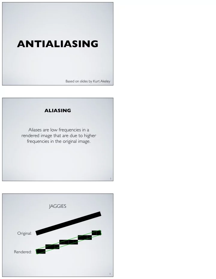
JAGGIES
Original: Rendered:
3
ANTIALIASING Based on slides by Kurt Akeley ALIASING Aliases are - - PDF document
ANTIALIASING Based on slides by Kurt Akeley ALIASING Aliases are low frequencies in a rendered image that are due to higher frequencies in the original image. 2 JAGGIES Original: Rendered: 3 CONVOLUTION THEOREM Let f and g be the
Based on slides by Kurt Akeley
ALIASING Aliases are low frequencies in a rendered image that are due to higher frequencies in the original image.
2
JAGGIES
Original: Rendered:
3
CONVOLUTION THEOREM
Let f and g be the transforms of f and g. Then Something difficult to do in one domain (e.g., convolution) may be easy to do in the other (e.g., multiplication)
4
ALIASED SAMPLING OF A POINT (OR LINE)
x
F(s) f(x)
5
ALIASED RECONSTRUCTION OF A POINT (OR LINE)
x
F(s) f(x) sinc(x)
6
RECONSTRUCTION ERROR (ACTUALLY NONE!)
Original Signal Aliased Reconstruction This is a special case!
7
RECONSTRUCTION ERROR
8
x
F(s) f(x)
Fourier theory explains jaggies as aliasing. For correct reconstruction:
! Signal must be band-limited ! Sampling must be at or above Nyquist rate ! Reconstruction must be done with a sinc function
All of these are difficult or impossible in the general case. Let’s see why …
9
Band-limiting changes (spreads) geometry
! Finite spectrum ! infinite spatial extent
Interferes with occlusion calculations Leaves visible seams between adjacent triangles Can’t band-limit the final image
! There is no final image, there are only samples ! If the sampling is aliased, there is no recovery
Nyquist-rate sampling requires band-limiting
10
In theory:
! Required sinc function has ! Negative lobes (displays can’t produce negative light) ! Infinite extent (cannot be implemented)
In practice:
! Reconstruction is done by a combination of ! Physical display characteristics (CRT, LCD, …) ! The optics of the human eye ! Mathematical reconstruction (as is done, for example, in high-
end audio equipment) is not practical at video rates.
11
TWO ANTIALIASING APPROACHES ARE PRACTICED
Pre-filtering
! Band-limit primitives prior to sampling ! OpenGL ‘smooth’ antialiasing
Increased sample rate
! Multisampling, super-sampling, distributed raytracing ! OpenGL ‘multisample’ antialiasing ! Effectively sampling above the Nyquist limit
12
13
IDEAL POINT (OR LINE CROSS SECTION)
x
F(s) f(x) sinc(x) sinc(x)
14
BAND-LIMITED UNIT DISK
x
F(s) f(x) sinc(x) sinc(x)
15
ALMOST-BAND-LIMITED UNIT DISK
x
F(s) f(x) sinc(x) sinc2(x)
Finite extent!
sinc3(x)
16
These are equivalent:
! Low-pass filtering ! Band-limiting ! (Ideal) reconstruction
These are equivalent:
! Point sampling of band-limited geometry ! Weighted area sampling of full-spectrum geometry
Sampled area Output pixel
17
Pros
! Almost eliminates aliasing due to undersampling ! Allows pre-computation of expensive filters ! Great image quality (with some caveats!)
Cons
! Can’t handle interactions of primitives with area ! Reconstruction is still a problem
18
PRE-FILTER POINT RASTERIZATION
alpha channel point being sampled at the center of this pixel
19
PRE-FILTER LINE RASTERIZATION
point being sampled at the center of this pixel alpha channel
20
http://people.csail.mit.edu/ericchan/articles/prefilter/ 21
http://people.csail.mit.edu/ericchan/articles/prefilter/ 22
Three arbitrary vertex locations define a huge parameter space Edges can be treated independently
! But this is a poor approximation near vertexes, where two or
three edges affect the filtering
! And triangles can be arbitrarily small
23
Solution: Weight fragments’ contributions according to the area they cover (Similar to alpha blending)
24
25
Two approaches to antialiasing
! Pre-filter ! Over-sample: increase sample rate
Pre-filter
! Works well for points and lines, not for triangles ! Can’t reasonably represent pre-filtered triangles ! Can’t handle occlusion ! Can effectively eliminate aliasing with a moderately-large filter
window Over-sample
! Works well for all primitives ! Though less well than pre-filtering for points and lines ! Cannot eliminate aliasing! ! Let’s see why …
26
Imperfect analogy, but useful pedagogical tool:
! Fundamental: spatial density of edges ! Harmonics: spectrum introduced by a single edge
Over-sampling cannot overcome increased fundamental frequency But over-sampling, followed by a resampling at a lower rate, can overcome harmonics due to a single edge
27
Low LOD Medium LOD High LOD
28
Over-sample to reduce jaggies due to edges
! Optimize for the case of a single edge
Use other approaches to limit edge rates
! Band-limit fundamental geometric frequencies ! Band-limit image fundamentals and harmonics
29
30
Supersampling algorithm:
31
SAMPLE AT 4X PIXEL RATE
x
F(s) f(x)
Pixel-rate fundamental
32
RECONSTRUCT 4X SAMPLES
x
F(s) f(x)
Cutoff at ! the over- sample rate Aliased !
33
BAND-LIMIT 4X RECONSTRUCTION TO PIXEL-RATE
x
F(s) f(x)
34
RESAMPLE AT PIXEL RATE
x
F(s) f(x)
35
RECONSTRUCT PIXEL SAMPLES
x
F(s) f(x)
Rect filter approximates LCD display
36
The over-sample reconstruction convolution and the band-limiting convolution steps can be combined:
! Convolution is associative ! (f * g) * h = f * (g * h) ! And g and h are constant ! f * (g * h) = f * filter
The filter convolution can be reduced to a simple weighted sum of sample values:
! The result is sampled at pixel rate ! So only values at pixel centers are needed ! These are weighted sums of the 4x samples
37
Do once
and band-limiting filters
the filter waveform During rendering:
filter weights During display
!
Reconstruct
38
39
40
Pattern categories
! Regular grid ! Random samples ! Pseudo-random (jittered grid)
Pattern variation
! Temporal ! Spatial
41
Implementation
! Regular sample spacing simplifies attribute
evaluation
! Mask, color, and depth ! Large sample count is expensive
Edge optimization
! Poor, especially for screen-aligned edges
Image quality
! Good for large numbers of samples
Single Pixel
42
Implementation
! Irregular sample spacing complicates attribute
evaluation
! Requires moderate sample size to avoid noise
Edge optimization
! Good, though less optimal for screen-aligned edges
Image quality
! Excellent for moderate numbers of samples
Temporal issues
! Must assign the same pattern to a given pixel in
each frame
Single Pixel random pattern
43
Implementation
! Best trade-off of sample number, noise level, and
anti-aliasing Temporal issues
! Must assign the same pattern to a given pixel in
each frame
random pattern
44
Supersampling does not eliminate aliasing
! It can reduce jaggies ! It must be used with other pre-filtering to eliminate
aliasing Multisampling
! Is supersampling with pixel-rate shading ! Optimized for efficiency and performance ! Is a full-scene antialiasing technique ! Works for all rendering primitives ! Handles occlusions correctly ! Can be used in conjunction with pre-filter antialiasing ! To optimize point and line quality
45
Two approaches to antialiasing are practiced
! Pre-filtering ! Multisampling
Pre-filter antialiasing
! Works well for non-area primitives (points, lines) ! Works poorly for area primitives (triangles, especially in 3-D)
Multisampling antialiasing
! Works well for all primitives ! Supersampling alone does not help--need to filter down to
pixel resolution
46
47
Eye’s resolution is not evenly distributed
! Foveal resolution is ~20x peripheral ! Systems can track direction of view, draw high-resolution inset ! Flicker sensitivity is higher in periphery
Human visual system is well engineered …
48
Ideal Actual
49
50
x
F(s) f(x)
51
FREQUENCIES ARE SELECTIVELY ATTENUATED
f(x) f(x)
52
SELECTIVE ATTENUATION (CONT.)
f(x) f(x)
53
MODULATION TRANSFER FUNCTION (MTF)
54
OPTICAL “IMPERFECTIONS” IMPROVE ACUITY
Image is pre-filtered
! Cutoff is approximately 60 cpd ! Cutoff is gradual – no ringing
Aliasing is avoided
! Foveal cone density is 120 / degree ! Cutoff matches retinal Nyquist limit
Vernier acuity is improved
! Foveal resolution is 30 arcsec ! Vernier acuity is 5-10 arcsec ! Linespread blur includes more sensors
55