Collision II, Antialiasing Week 11, Mon Mar 26 - PowerPoint PPT Presentation

University of British Columbia CPSC 314 Computer Graphics Jan-Apr 2007 Tamara Munzner Collision II, Antialiasing Week 11, Mon Mar 26 http://www.ugrad.cs.ubc.ca/~cs314/Vjan2007

News • Homework 4 out today • due Wed 11 Apr, 10am • extra TA office hours in lab for midterm Q&A • Tuesday 4pm Gordon • H3 solutions, graded H3 handed back • P4 proposal email feedback out to all who turned in • some were missing real email, used ugrad accounts 2

Midterm 2: Wed Mar 26 • covering through Homework 3 material • MT1: transformations, some viewing • MT2 emphasis • some viewing • projections • color • rasterization • lighting/shading • advanced rendering (incl raytracing) • graded H3 + solutions out Monday 3

Midterm 2: Wed Mar 26 • closed book • allowed to have • calculator • one side of 8.5”x11” paper, handwritten • write your name on it • turn it in with exam, you’ll get it back • have ID out and face up 4

Review: Select/Hit Picking • assign (hierarchical) integer key/name(s) • small region around cursor as new viewport • redraw in selection mode • equivalent to casting pick “tube” • store keys, depth for drawn objects in hit list • examine hit list • usually use frontmost, but up to application 5

Correction/Review: Hit List • glSelectBuffer(buffersize, *buffer) • where to store hit list data • on hit, copy entire contents of name stack to output buffer. • hit record • number of names on stack • minimum and maximum depth of object vertices • depth lies in the z-buffer range [0,1] • multiplied by 2^32 -1 then rounded to nearest int 6

Review: Collision Detection • boundary check • perimeter of world vs. viewpoint or objects • 2D/3D absolute coordinates for bounds • simple point in space for viewpoint/objects • set of fixed barriers • walls in maze game • 2D/3D absolute coordinate system • set of moveable objects • one object against set of items • missile vs. several tanks • multiple objects against each other • punching game: arms and legs of players • room of bouncing balls 7

Reading for Collision/Acceleration • FCG Sect 10.9 Sub-Linear 8

Collision/Acceleration II 9

Accelerating Collision Detection • two kinds of approaches (many others also) • collision proxies / bounding volumes • spatial data structures to localize • used for both 2D and 3D • used to accelerate many things, not just collision detection • raytracing • culling geometry before using standard rendering pipeline 10

Collision Proxies • proxy: something that takes place of real object • cheaper than general mesh-mesh intersections • collision proxy (bounding volume) is piece of geometry used to represent complex object for purposes of finding collision • if proxy collides, object is said to collide • collision points mapped back onto original object • good proxy: cheap to compute collisions for, tight fit to the real geometry • common proxies: sphere, cylinder, box, ellipsoid • consider: fat player, thin player, rocket, car … 11

Trade-off in Choosing Proxies Sphere OBB AABB 6-dop Convex Hull increasing complexity & tightness of fit decreasing cost of (overlap tests + proxy update) • AABB: axis aligned bounding box • OBB: oriented bounding box, arbitrary alignment • k-dops – shapes bounded by planes at fixed orientations • discrete orientation polytope 12

Pair Reduction • want proxy for any moving object requiring collision detection • before pair of objects tested in any detail, quickly test if proxies intersect • when lots of moving objects, even this quick bounding sphere test can take too long: N 2 times if there are N objects • reducing this N 2 problem is called pair reduction • pair testing isn’t a big issue until N>50 or so… 13

Spatial Data Structures • can only hit something that is close • spatial data structures tell you what is close to object • uniform grid, octrees, kd-trees, BSP trees • bounding volume hierarchies • OBB trees • for player-wall problem, typically use same spatial data structure as for rendering • BSP trees most common 14

Uniform Grids • axis-aligned • divide space uniformly 15

Quadtrees/Octrees • axis-aligned • subdivide until no points in cell 16

KD Trees • axis-aligned • subdivide in alternating dimensions 17

BSP Trees • planes at arbitrary orientation 18

Bounding Volume Hierarchies 19

OBB Trees 20

Related Reading • Real-Time Rendering • Tomas Moller and Eric Haines • on reserve in CICSR reading room 21

Acknowledgement • slides borrow heavily from • Stephen Chenney, (UWisc CS679) • http://www.cs.wisc.edu/~schenney/courses/cs679-f2003/lectures/cs679-22.ppt • slides borrow lightly from • Steve Rotenberg, (UCSD CSE169) • http://graphics.ucsd.edu/courses/cse169_w05/CSE169_17.ppt • further reading: Real-Time Rendering • Tomas Moller and Eric Haines • on reserve in CICSR reading room 22

Antialiasing 23

Reading for Antialiasing • FCG Sec 3.7 Simple Antialiasing • FCG Sec 10.11.1 Antialiasing • FCG Chap 4 Signal Processing (optional) 24

Samples • most things in the real world are continuous • everything in a computer is discrete • the process of mapping a continuous function to a discrete one is called sampling • the process of mapping a discrete function to a continuous one is called reconstruction • the process of mapping a continuous variable to a discrete one is called quantization • rendering an image requires sampling and quantization • displaying an image involves reconstruction 25

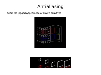
Jaggy Line Segments • we tried to sample a line segment so it would map to a 2D raster display • we quantized the pixel values to 0 or 1 • we saw stairsteps / jaggies 26

Less Jaggy Line Segments • better if quantize to many shades • image is less visibly jaggy • find color for area, not just single point at center of pixel • supersampling: sample at higher frequency than intended display size 27

Supersample and Average • supersample: create image at higher resolution • e.g. 768x768 instead of 256x256 • shade pixels wrt area covered by thick line/rectangle • average across many pixels • e.g. 3x3 small pixel block to find value for 1 big pixel • rough approximation divides each pixel into a finer grid of pixels 5/9 9/9 9/9 6/9 4/9 0/9 28

Supersample and Average • supersample: jaggies less obvious, but still there • small pixel center check still misses information • unweighted area sampling • equal areas cause equal intensity, regardless of distance from pixel center to area • aka box filter Intensity W(x,y) 5/9 9/9 9/9 6/9 4/9 0/9 x 29

Supersampling Example: Image 3x3 supersampling with no supersampling 3x3 unweighted filter 30

Weighted Area Sampling • intuitively, pixel cut through the center should be more heavily weighted than one cut along corner • weighting function, W(x,y) • specifies the contribution of primitive passing through the point (x, y) from pixel center • Gaussian filter (or approximation) commonly used Intensity W(x,y) x 31

Sampling Errors • some objects missed entirely, others poorly sampled • could try unweighted or weighted area sampling • but how can we be sure we show everything? • need to think about entire class of solutions! • brief taste of signal processing (Chap 4 FCG) 32

Image As Signal • image as spatial signal • 2D raster image • discrete sampling of 2D spatial signal • 1D slice of raster image • discrete sampling of 1D spatial signal Intensity Pixel position across scanline Examples from Foley, van Dam, Feiner, and Hughes 33

Sampling Frequency • if don’t sample often enough, resulting signal misinterpreted as lower-frequency one • we call this aliasing Examples from Foley, van Dam, Feiner, and Hughes 34

Sampling Theorem continuous signal can be completely recovered from its samples iff sampling rate greater than twice maximum frequency present in signal - Claude Shannon 35

Nyquist Rate • lower bound on sampling rate • twice the highest frequency component in the image’s spectrum 36

Aliasing • incorrect appearance of high frequencies as low frequencies • to avoid: antialiasing • supersample • sample at higher frequency • low pass filtering • remove high frequency function parts • aka prefiltering, band-limiting 37

Low-Pass Filtering Examples from Foley, van Dam, Feiner, and Hughes 38

Low-Pass Filtering Examples from Foley, van Dam, Feiner, and Hughes 39

Filtering • low pass • blur • high pass • edge finding 40

Texture Antialiasing • texture mipmapping: low pass filter 41

Temporal Antialiasing • subtle point: collision detection about algorithms for finding collisions in time as much as space • temporal sampling • aliasing: can miss collision completely with point samples! • temporal antialiasing • test line segment representing motion of object center 42