Rev eview iew of of Probabilit obability Theor heory and and - PDF document
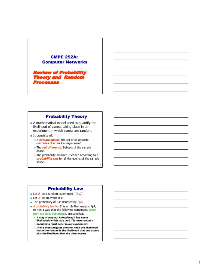
CMPE 252A: Computer Networks Rev eview iew of of Probabilit obability Theor heory and and Random andom Proces ocesses es 1 Probability Theory A mathematical model used to quantify the likelihood of events taking place in an
CMPE 252A: Computer Networks Rev eview iew of of Probabilit obability Theor heory and and Random andom Proces ocesses es 1 Probability Theory A mathematical model used to quantify the likelihood of events taking place in an experiment in which events are random. It consists of: A sample space : The set of all possible outcomes of a random experiment . The set of events : Subsets of the sample space. The probability measure: Defined according to a probability law for all the events of the sample space. 2 Probability Law Let E be a random experiment (r.e.) Let A be an event in E The probability of A is denoted by P(A) A probability law for E is a rule that assigns P(A) to A in a way that the following conditions, taken from our daily experience, are satisfied : A may or may not take place; it has some likelihood (which may be 0 if it never occurs). Something must occur in our experiment. If one event negates another, then the likelihood that either occurs is the likelihood that one occurs plus the likelihood that the other occurs. 3 1
Probability Law More formally, we state the same as follows. A probability law for E is a rule that assigns a number P(A) to each event A in E satisfying the following axioms: AI: 0 ≤ P(A) AII: P ( S ) 1 = AIII: A B P ( A B ) P(A) P(B) = φ ⇒ = + Everything else is derived from these axioms! 4 Important Corollaries 1. A , A , ... A A A i j P ( A ) P ( A ) = Φ ∀ ≠ ⇒ = ∑ 1 2 n i j k k k k 2. P ( A c ) 1 P ( A ) = − 3. P ( A ) 1 ≤ 4. P ( ) 0 Φ = 5. P ( A B ) P ( A ) P ( B ) P ( A B ) = + − 5 Probability Law 1 P ( S ) = S P ( A ) A P ( x ) x Φ 0 = P ( ) Φ All probabilities must be in [0, 1] The sum of probabilities must be at most 1 6 2
Conditional Probability Events of interest occur within some context, and that context changes their likelihood. time packet collisions time interarrival times We are interested in events occurring given that others take place! 7 Conditional Probability The likelihood of an event A occurring given that another event B occurs is smaller than the likelihood that A occurs at all. We define the conditional probability of A given B as follows: P ( A B ) ∩ P ( A | B ) for P ( B ) 0 = > P ( B ) We require P(B) > 0 because we know B occurs! 8 Theorem of Total Probability Purpose is to divide and conquer We can describe how likely an event is by partitioning it into mutually exclusive pieces. busy period idle period busy period success failure time B B B 1 2 3 9 3
Theorem of Total Probability B B 3 1 A B 2 A ∩ B 2 B ... n Intersections of A with B ’ s are mutually exclusive P ( A ) P ( A | B ) P ( B ) P ( A B ) ∑ ∑ = = ∩ i i i i i 10 Independence of Events In many cases, an event does not depend on prior events, or we want that to be the case. Example: Our probability model should not have to account for the entire history of a LAN. Independence of an even with respect to another means that its likelihood does not depend on that other event. A is independent of B if P(A | B) = P(A) B is independent of A if P(B | A) = P(B) So the likelihood of A does not change by knowing about B and viceversa! This also means: P ( A B ) P ( A ) P ( B ) ∩ = 11 Random Variables We are not interested in describing the likelihood of every outcome of an experiment explicitly. We are interested in quantitative properties associated with the outcomes of the experiment. Example: What is the probability with which each packet sent in an experiment is received correctly? We don ’ t really care! What is the probability of receiving no packets correctly within a period of T sec.? We care! This may make a router delete a neighbor! 12 4
Random Variables We implicitly use a measurement that assigns a numerical value to each outcome of the experiment. The measurement is [in theory] deterministic; based on deterministic rules. The randomness of the observed values of the measurement is completely determined by the randomness of the experiment itself. A random variable X is a rule that assigns a numerical value to each outcome of a random experiment Yes, it is really a function! 13 Random Variables Definition: A random variable X on a sample space S is a function X: S ->R that assigns a real number X(s) to each sample point s in S. S s s s s s 5 1 3 2 4 − ∞ + ∞ X ( 1 s ) X ( 2 s ) X ( s ) X ( s ) 0 = 4 5 S { X ( s ) | s S } = ∈ ⊂ ℜ which is called the event space X i i 14 Random Variables Purpose is to simplify the description of the problem. We will not have to define the sample space! 1 S s P ( X ( s ) x ) = 0 X ( s ) x − ∞ = + ∞ Possible values of X 15 5
Types of Random Variables Discrete and continuous: Typically used for counting packets or measuring time intervals. 1 2 3 4 time t 0 next packet Busy period time time? 16 Discrete Random Variables We are interested in the probability that a discrete random variable X (our measurement!) equals a certain value or range of values. Example: We measure the delay experienced by each packet sent from one host to another over the Internet; say we sent 1M packets (we have 1M delay measurements). We want to know the likelihood with which any one packet experiences a delay of 5 ms or less. Probability Mass Function ( pmf ) of a random variable X : The probability that X assumes a given value x P ( X x ) p ( x ) = = X 17 Discrete Random Variables Cumulative Distribution Function (cdf) of a random variable X : The probability that X takes on any value in the interval ( , x ] −∞ F X ( x ) P ( X x ) = ≤ The pdf and pmf of a random variable are just probabilities and obey the same axioms AI to AIII. Therefore, 0 F ( x ) 1 ; lim F ( x ) 1 ; lim F ( x ) 0 ≤ ≤ = = X x X X → + ∞ x → −∞ F ( a ) F ( b ) for a b ≤ < X X P(a X b) F ( b ) F ( a ) < ≤ = − X X 18 6
Continuous Random Variables The probability that a continuous r.v. X assumes a given value is 0. Therefore, we use the probability that X assumes a range of values and make that length of that range tend to 0. The probability density function ( pdf ) of X , if it exists, is defined in terms of the cdf of X as dF ( x ) f ( x ) X = X dx b x P(a X b) f (x)dx ; F ( x ) f ( t ) dt P ( X x ) ≤ ≤ = ∫ = ∫ = − ∞ ≤ ≤ X X X a − ∞ + ∞ if x then f ( t ) dt 1 , because pdf is a probabilit y → + ∞ ∫ = X − ∞ 19 What We Will Use We are interested in: Using the definitions of well-known r.v.s to compute probabilities Computing average values and deviations from those values for well-known r.v.s 20 Mean and Variance VC2 2 6 A 7 B 5 1 C 3 4 D VC1 For VC1 use 3 For VC2 use 2 What is the average queue length at each ….. router? For VCn use 3 What is our worst case queue? 21 7
Mean and Variance Expected value or mean of X: E ( X ) x p ( k ) for d.r.v. ∑ = k X k + ∞ E ( X ) tf ( t ) dt for c.r.v = ∫ X − ∞ Mean is always defined for us! queue size too much? mean time 22 Variance Describes how much a r.v. deviates from its average value, i.e., D = X - E(X) We are only interested in the magnitude of the deviation, so we use: D 2 ( X E ( X )) 2 = − The variance of a r.v. is defined as the mean squared variation 2 E ( D ) Var ( X ) 2 E ([ X E ( X )] 2 ) = σ = − Important relation: 2 2 Var ( X ) E ( X ) E ( X ) = − 23 Properties of Mean and Variance E ( aX b ) aE ( X ) b ; E ( b ) b + = + = Var ( c ) 0 = Var ( X c ) Var ( X ) + = 2 Var ( cX ) c Var ( X ) = Useful when we discuss amplifying random variables or adding constant biases. 24 8
Examples of Random Variables We are interested in those r.v. that permit us to model system behavior based on the present state alone. We need to count arrivals in a time interval count the number of times we need to repeat something to succeed count the number of successes and failures measure the time between consecutive arrivals The trick is to map our performance questions into the above four types of experiments 25 Bernoulli Random Variable Let A be an event related to the outcomes of a random experiment. X = 1 if outcome occurs and 0 otherwise This is the Bernoulli r.v. and has two possible outcomes: success (1) or failure (0) P ( 0 ) P P ( X 0 ) q 1 p = = = = = − X 0 P ( 1 ) P P ( X 1 ) p 1 q = = = = = − X 1 We use it as a building block for other types of counting 26 Geometric Random Variable Used to count the number of attempts needed to succeed doing something. Example: How many times do we have to transmit a packet over a broadcast radio channel before it is sent w/o interference? time failure failure failure success! Assume that each attempt is independent of any prior attempt! Assume each attempt has the same probability of success ( p ) 27 9
Recommend
More recommend
Explore More Topics
Stay informed with curated content and fresh updates.

