Reminder of Asymptotic Notation Let f , g : N ! R be functions. We - PowerPoint PPT Presentation

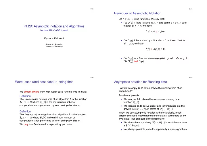
1 / 18 2 / 18 Reminder of Asymptotic Notation Let f , g : N ! R be functions. We say that: I f is O ( g ) if there is some n 0 2 N and some c > 0 2 R such that for all n � n 0 we have Inf 2B: Asymptotic notation and Algorithms Lecture 2B of ADS thread 0  f ( n )  c g ( n ) . Kyriakos Kalorkoti I f is Ω ( g ) if there is an n 0 2 N and c > 0 in R such that for all n � n 0 we have School of Informatics University of Edinburgh f ( n ) � c g ( n ) � 0 . I f f f is Θ ( g ) , or f has the same asymptotic growth rate as g , if f is O ( g ) and Ω ( g ) . 3 / 18 4 / 18 Worst-case (and best-case) running-time Asymptotic notation for Running-time How do we apply O , Ω , Θ to analyse the running-time of an algorithm A? We almost always work with Worst-case running time in Inf2B: Possible approach: Definition I We analyse A to obtain the worst-case running time The (worst-case) running time of an algorithm A is the function T A : N ! N where T A ( n ) is the maximum number of function T A ( n ) . computation steps performed by A on an input of size n . I We then go on to derive upper and lower bounds on (the � � � � growth rate of) T A ( n ) , in terms of O · · , Ω . Definition In fact we use asymptotic notation with the analysis, much The (best-case) running time of an algorithm A is the function simpler (no need to give names to constants, takes care of low B A : N ! N where B A ( n ) is the minimum number of level detail that isn’t part of the big picture). computation steps performed by A on an input of size n . I We aim to have matching O � � � � · · , Ω bounds hence have We only use Best-case for explanatory purposes. � � a Θ · bound. I Not always possible, even for apparently simple algorithms.

5 / 18 6 / 18 Example linSearch Input: Integer array A , integer k being searched. Output: The least index i such that A [ i ] = k . algA(A,r,s) algB(A,r,s) 1. if r < s then 1. if A [ r ] < A [ s ] then Algorithm linSearch ( A , k ) 2. for i r to s do 2. swap A [ r ] with A [ s ] 1. for i 0 to A . length � 1 do 3. for j i to s do 3. if r < s � r then m b i + j 2. if A [ i ] = k then 2 c algA ( A , r , s � r ) 4. 4. 3. return i 5. algB ( A , i , m � 1 ) 4. return � 1 6. algB ( A , m , j ) m b r + s 7. 2 c (Lecture Note 1) Worst-case running time T linSearch ( n ) satisfies 8. algA ( A , r , m � 1 ) 9. algA ( A , m , s ) ( c 1 + c 2 ) n + min { c 3 , c 1 + c 4 }  T linSearch ( n )  ( c 1 + c 2 ) n + max { c 3 , c 1 + c 4 } . Best-case running time satisfies B linSearch ( n ) = c 1 + c 2 + c 3 . 7 / 18 8 / 18 Picture of T linSearch ( n ) , B linSearch ( n ) T linSearch ( n ) = O ( n ) Proof. 70 T(n)=(c +c )n + ... From Lecture Note 1 we have 65 1 2 60 � 55 T linSearch ( n )  ( c 1 + c 2 ) · n + max c 3 , ( c 1 + c 4 ) . 50 45 40 Take n 0 = max { c 3 , ( c 1 + c 4 ) } , c = c 1 + c 2 + 1. 35 30 Then for every n � n 0 , we have 25 20 T linSearch ( n )  ( c 1 + c 2 ) n + n 0 15 10  ( c 1 + c 2 + 1 ) n = cn . B(n)=c +c +c 5 1 2 3 5 10 15 20 25 30 35 40 45 Hence T linSearch ( n ) = O ( n ) .

9 / 18 10 / 18 T linSearch ( n ) = Ω ( n ) Misconceptions/Myths about O and Ω We know T linSearch ( n ) = O ( n ) . Also true: T linSearch ( n ) = O ( n lg ( n )) , T linSearch ( n ) = O ( n 2 ) . M ISCONCEPTION 1 Is T linSearch ( n ) = O ( n ) the best we can do? If we can show T A ( n ) = O ( f ( n )) for some function f : N ! R , then the running time of A on inputs of YES, because . . . size n is bounded by f ( n ) for sufficiently large n . T linSearch ( n ) = Ω ( n ) . FALSE: Only guaranteed an upper bound of cf ( n ) , for some Proof. constant c > 0. T linSearch ( n ) � ( c 1 + c 2 ) n , because all c i are positive. Example: Consider linSearch. We could have shown Take n 0 = 1 and c = c 1 + c 2 in defn of Ω . T linSearch = O ( 1 2 ( c 1 + c 2 ) n ) (or O ( α n ) , for any constant α > 0) exactly as we showed T linSearch ( n ) = O ( n ) but . . . T linSearch ( n ) = Θ ( n ) . the worst-case for linSearch is greater than 1 2 ( c 1 + c 2 ) n . 11 / 18 12 / 18 Misconceptions/Myths about O and Ω Insertion Sort Input: An integer array A M ISCONCEPTION 2 Output: Array A sorted in non-decreasing order Because T A ( n ) = O ( f ( n )) implies a c f ( n ) upper bound on the running-time of A for all inputs of size n , Algorithm insertionSort ( A ) then T A ( n ) = Ω ( g ( n )) implies a similar lower bound on 1. for j 1 to A . length � 1 do the running-time of A for all inputs of size n . 2. a A [ j ] i j � 1 3. FALSE: If T A ( n ) = Ω ( g ( n )) for some g : N ! R , then there is 4. while i � 0 and A [ i ] > a do some constant c 0 > 0 such that T A ( n ) � c 0 g ( n ) for all 5. A [ i + 1 ] A [ i ] sufficiently large n . 6. i i � 1 But A can be much faster than T A ( n ) on other inputs of length n 7. A [ i + 1 ] a that are not worst-case! No lower bound on general inputs of size n . linSearch graph is an example.

13 / 18 14 / 18 Example: Insertion Sort Big-O for T insertionSort ( n ) Input: 3 6 5 1 4 Algorithm insertionSort ( A ) 1. for j 1 to A . length � 1 do j=1 3 6 5 1 4 2. a A [ j ] 3. i j � 1 4. while i � 0 and A [ i ] > a do j=2 5 6 3 6 5 1 4 A [ i + 1 ] A [ i ] 5. 6. i i � 1 7. A [ i + 1 ] a j=3 1 3 5 6 3 5 6 1 4 Line 1 O ( 1 ) time, executed A . length � 1 = n � 1 times. Lines 2,3,7 O ( 1 ) time each, executed n � 1 times. Lines 4,5,6 O ( 1 ) -time, executed together as for -loop. No. of executions depends on for -test, j . j=4 1 3 4 5 6 5 6 4 For fixed j , for -loop at 4. takes at most j iterations. 15 / 18 16 / 18 T insertionSort ( n ) = Ω ( n 2 ) Algorithm insertionSort ( A ) Harder than O ( n 2 ) bound. 1. for j 1 to A . length � 1 do a A [ j ] 2. Focus on a BAD instance of size n : 3. i j � 1 Take input instance h n , n � 1 , n � 2 , . . . , 2 , 1 i . 4. while i � 0 and A [ i ] > a do I For every j = 1 . . . , n � 1, insertionSort uses j executions 5. A [ i + 1 ] A [ i ] of line 5 to insert A [ j ] . 6. i i � 1 Then A [ i + 1 ] a 7. n � 1 For a fixed j , lines 2-7 take at most X T insertionSort ( n ) � c j O ( 1 )+ O ( 1 ) + O ( 1 ) + O ( j ) + O ( j ) + O ( j ) + O ( 1 ) j = 1 = O ( 1 ) + O ( j ) n � 1 c n ( n � 1 ) X = c j = = O ( 1 ) + O ( n ) . 2 j = 1 = O ( n ) . So T insertionSort ( n ) = Ω ( n 2 ) and T insertionSort ( n ) = Θ ( n 2 ) . There are n � 1 different j -values. Hence T insertionSort ( n ) = ( n � 1 ) O ( n ) = O ( n ) O ( n ) = O ( n 2 ) .

17 / 18 18 / 18 “Typical” asymptotic running times Further Reading I Θ ( lg n ) (logarithmic), I Lecture notes 2 from last week. I Θ ( n ) (linear), I If you have Goodrich & Tamassia [GT]: I Θ � � n lg n (n-log-n), All of the chapter on “Analysis Tools” (especially the I Θ ( n 2 ) (quadratic), “Seven functions” and “Analysis of Algorithms” sections). I If you have [CLRS]: I Θ ( n 3 ) (cubic), Read chapter 3 on “Growth of Functions.” I Θ ( 2 n ) (exponential).