Asymptotic Analysis Pedro Ribeiro DCC/FCUP 2018/2019 Pedro - PowerPoint PPT Presentation

Asymptotic Analysis Pedro Ribeiro DCC/FCUP 2018/2019 Pedro Ribeiro (DCC/FCUP) Asymptotic Analysis 2018/2019 1 / 79

Motivational Example - TSP Traveling Salesman Problem (Euclidean TSP version) Input : a set S of n points in the plane Output : the smallest possible path that starts on a point, visits all other points of S and then returns to the starting point. An example: Pedro Ribeiro (DCC/FCUP) Asymptotic Analysis 2018/2019 2 / 79

Motivational Example - TSP A possible (greedy) algorithm - nearest neighbour p 1 ← random point i ← 1 While (there are still points to visit) do i ← i + 1 p i ← nearest non visited neighbour of point p i − 1 return path p 1 → p 2 → . . . → p n → p 1 Pedro Ribeiro (DCC/FCUP) Asymptotic Analysis 2018/2019 3 / 79

Motivational Example - TSP Seems to work... ⇒ Pedro Ribeiro (DCC/FCUP) Asymptotic Analysis 2018/2019 4 / 79

Motivational Example - TSP But it is does not work for all instances! (Note: starting with the leftmost point would not solve the problem) Pedro Ribeiro (DCC/FCUP) Asymptotic Analysis 2018/2019 5 / 79

Motivacional Example - TSP Another possible (greedy) algorithm For i ← 1 to ( n − 1) do Add connection between closest pair of points such that they are in different connected components Add connection between the two ”extremes” of the created path return the cyclic path created Pedro Ribeiro (DCC/FCUP) Asymptotic Analysis 2018/2019 6 / 79

Motivational Example - TSP It does not work for all cases! Pedro Ribeiro (DCC/FCUP) Asymptotic Analysis 2018/2019 7 / 79

Motivational Example - TSP How to solve the problem then? A possible algorithm (exhaustive search a.k.a. ”brute force”) P min ← any permutation of the points in S For P i ← each of the permutations of points in S If ( cost ( P i ) < cost ( P min )) then P min ← P i retorn Path formed by P min A correct algorithm, but extremely slow! P ( n ) = n ! = n × ( n − 1) × . . . × 1 For instance, P (20) = 2 , 432 , 902 , 008 , 176 , 640 , 000 For a set of 20 points, even the fastest computer in the world would not solve it! (how long would it take?) Pedro Ribeiro (DCC/FCUP) Asymptotic Analysis 2018/2019 8 / 79

Motivational Example - TSP The present problem is a restricted version (euclidean) of one of the most well known ”classic” hard problems, the Travelling Salesman Problem ( TSP ) This problem has many possible applications Ex: genomic analysis, industrial production, vehicle routing, ... There is no known efficient solution for this problem (with optimal results, not just approximated) The presented solution has O ( n !) complexity The Held-Karp algorithm has O (2 n n 2 ) complexity (this notation will be the focus of this class) TSP belongs to the class of NP-hard problems The decision version belongs to the class of NP-complete problems (we will also talk about this at the end of the semester) Pedro Ribeiro (DCC/FCUP) Asymptotic Analysis 2018/2019 9 / 79

An experience - how many instructions How many instructions per second on a current computer? (just an approximation, an order of magnitude) On my notebook, about 10 9 instructions At this velocity, how much time for the following quantities of instructions? Quant. 100 1000 10000 N < 0 . 01 s < 0 . 01 s < 0 . 01 s N 2 < 0 . 01 s < 0 . 01 s 0 . 1 s N 3 < 0 . 01 s 1 . 00 s 16 min N 4 0 . 1 s 16 min 115 days 10 13 years 10 284 years 10 2993 years 2 N 10 141 years 10 2551 years 10 35642 years n ! Pedro Ribeiro (DCC/FCUP) Asymptotic Analysis 2018/2019 10 / 79

An experience: - Permutations Let’s go back to the idea of permutations Exemple: the 6 permutations of { 1 , 2 , 3 } 1 2 3 1 3 2 2 1 3 2 3 1 3 1 2 3 2 1 Recall that the number of permutations can be computed as: P ( n ) = n ! = n × ( n − 1) × . . . × 1 (do you understand the intuition on the formula?) Pedro Ribeiro (DCC/FCUP) Asymptotic Analysis 2018/2019 11 / 79

An experience: - Permutations What is the execution time of a program that goes through all permutations? (the following times are approximated, on my notebook) (what I want to show is order of growth ) n ≤ 7 : < 0 . 001 s n = 8 : 0 . 001 s n = 9 : 0 . 016 s How many permutations per second? n = 10 : 0 . 185 s About 10 7 n = 11 : 2 . 204 s n = 12 : 28 . 460 s . . . n = 20 : 5000 years ! Pedro Ribeiro (DCC/FCUP) Asymptotic Analysis 2018/2019 12 / 79

On computer speed Will a faster computer be of any help? No! If n = 20 → 5000 years, hypothetically: ◮ 10x faster would still take 500 years ◮ 5,000x would still take 1 year ◮ 1,000,000x faster would still take two days, but n = 21 would take more than a month n = 22 would take more than a year! The growth rate of the execution time is what matters! Algorithmic performance vs Computer speed A better algorithm on a slower computer will always win against a worst algorithm on a faster computer, for sufficiently large instances Pedro Ribeiro (DCC/FCUP) Asymptotic Analysis 2018/2019 13 / 79

Why worry? What can we do with execution time/memory analysis? Prediction How much time/space does an algorithm need to solve a problem? How does it scale? Can we provide guarantees on its running time/memory? Comparison Is an algorithm A better than an algorithm B ? Fundamentally, what is the best we can possibly do on a certain problem? We will study a methodology to answer these questions We will focus mainly on execution time analysis Pedro Ribeiro (DCC/FCUP) Asymptotic Analysis 2018/2019 14 / 79

Random Access Machine (RAM) We need a model that is generic and independent from the language and the machine. We will consider a Random Access Machine (RAM) ◮ Each simple operation (ex: +, − , ← , If ) takes 1 step ◮ Loops and procedures, for example, are not simple instructions! ◮ Each access to memory takes also 1 step We can measure execution time by... counting the number of steps as a function of the input size n : T ( n ). Operations are simplified , but this is useful Ex: summing two integers does not cost the same as dividing two reals, but we will see that on a global vision, these specific values are not important Pedro Ribeiro (DCC/FCUP) Asymptotic Analysis 2018/2019 15 / 79

Random Access Machine (RAM) A counting example A simple program int count = 0; for ( int i=0; i<n; i++) if (v[i] == 0) count++ Let’s count the number of simple operations: Variable declarations 2 Assignments: 2 ”Less than” comparisons n + 1 ”Equality” comparisons: n Array access n Increment between n and 2 n Pedro Ribeiro (DCC/FCUP) Asymptotic Analysis 2018/2019 16 / 79

Random Access Machine (RAM) A counting example A simple program int count = 0; for ( int i=0; i<n; i++) if (v[i] == 0) count++ Total number of steps on the worst case: T ( n ) = 2 + 2 + ( n + 1) + n + n + 2 n = 5 + 5 n Total number of steps on the best case: T ( n ) = 2 + 2 + ( n + 1) + n + n + n = 5 + 4 n Pedro Ribeiro (DCC/FCUP) Asymptotic Analysis 2018/2019 17 / 79

Types of algorithm analysis Worst Case analysis: (the most common) T ( n ) = maximum amount of time for any input of size n Average Case analysis: (sometimes) T ( n ) = average time on all inputs of size n Implies knowing the statistical distribution of the inputs Best Case analysis: (”deceiving”) It’s almost like ”cheating” with an algorithm that is fast just for some of the inputs Pedro Ribeiro (DCC/FCUP) Asymptotic Analysis 2018/2019 18 / 79

Types of algorithm analysis Pedro Ribeiro (DCC/FCUP) Asymptotic Analysis 2018/2019 19 / 79

Asymptotic Notation We need a mathematical tool to compare functions On algorithm analysis we use Asymptotic Analysis : ”Mathematically”: studying the behaviour of limits (as n → ∞ ) Computer Science: studying the behaviour for arbitrary large input or ”describing” growth rate A very specific notation is used: O , Ω , Θ , o , ω It allows to focus on orders of growth Pedro Ribeiro (DCC/FCUP) Asymptotic Analysis 2018/2019 20 / 79

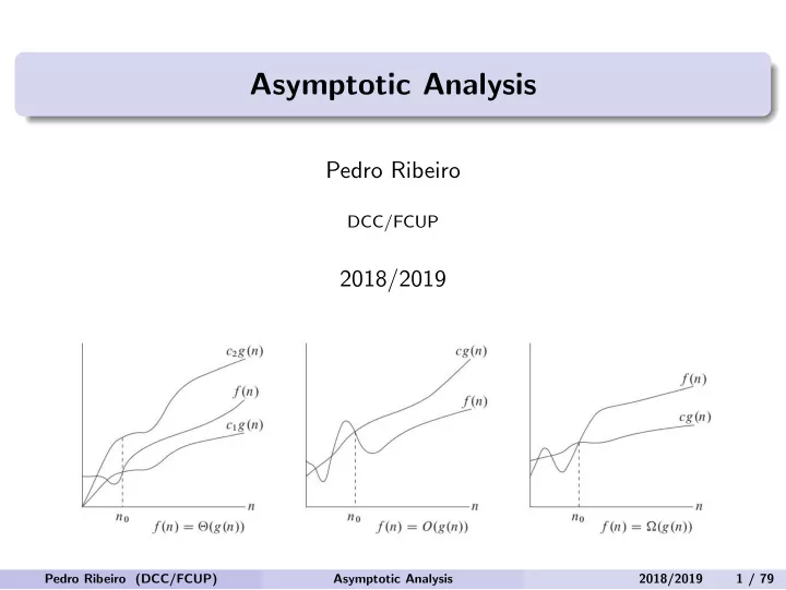
Asymptotic Notation Definitions f ( n ) = O ( g ( n )) It means that c × g ( n ) is an upper bound of f ( n ) f ( n ) = Ω ( g ( n )) It means that c × g ( n ) is a lower bound of f ( n ) f ( n ) = Θ ( g ( n )) It means that c 1 × g ( n ) is a lower bound of f ( n ) and c 2 × g ( n ) is an upper bound of f ( n ) Note: ∈ could be used instead of = Pedro Ribeiro (DCC/FCUP) Asymptotic Analysis 2018/2019 21 / 79

Asymptotic Notation A graphical depiction Θ O Ω The definitions imply an n from which the function is bounded. The small values of n do not ”matter”. Pedro Ribeiro (DCC/FCUP) Asymptotic Analysis 2018/2019 22 / 79

Asymptotic Notation Formalization f ( n ) = O ( g ( n )) if there exist positive constants n 0 and c such that f ( n ) ≤ c × g ( n ) for all n ≥ n 0 f ( n ) = Ω ( g ( n )) if there exist positive constants n 0 and c such that f ( n ) ≥ c × g ( n ) for all n ≥ n 0 f ( n ) = Θ ( g ( n )) if there exist positive constants n 0 , c 1 and c 2 such that c 1 × g ( n ) ≤ f ( n ) ≤ c 2 × g ( n ) for all n ≥ n 0 f ( n ) = o ( g ( n )) if for any positive constant c there exists n 0 such that f ( n ) < c × g ( n ) for all n ≥ n 0 f ( n ) = ω ( g ( n )) if for any positive constant c there exists n 0 such that f ( n ) > c × g ( n ) for all n ≥ n 0 Pedro Ribeiro (DCC/FCUP) Asymptotic Analysis 2018/2019 23 / 79