Reliable and efficient model reduction of parametrized aerodynamics - PowerPoint PPT Presentation
Reliable and efficient model reduction of parametrized aerodynamics problems - error estimation and adaptivity Masayuki Yano University of Toronto Institute for Aerospace Studies Joint work with Eugene Du & Michael Sleeman Algorithms for
Reliable and efficient model reduction of parametrized aerodynamics problems - error estimation and adaptivity Masayuki Yano University of Toronto Institute for Aerospace Studies Joint work with Eugene Du & Michael Sleeman Algorithms for Dimension and Complexity Reduction ICERM, Providence, United States 27 March 2020
Acknowledgment Students: Eugene Du Michael Sleeman Acknowledgment: Anthony Patera Sponsors: Natural Sciences and Engineering Research Council of Canada Canada Foundation for Innovation SciNet
Motivation: parametrized aerodynamics problems Goal: rapid and reliable output prediction of parametrized nonlinear PDEs in many-query/real-time scenarios. PDEs: compressible (Reynolds-averaged) Navier-Stokes Many-query/real-time scenarios: parameter & design sweep uncertainty quantification unsteady flow prediction 1
Mathematical problem µ PDE: given µ ∈ D ⊂ R P , find u ( µ ) ∈ V s.t. ∇ · ( F ( u ( µ ); µ ) + K ( u ( µ ); µ ) ∇ u ( µ ) ) = S ( u ( µ ); µ ) � �� � � �� � � �� � advection flux diffusion flux source and evaluate output s ( µ ) ≡ q ( u ( µ ); µ ) . � �� � output functional Challenges: aerodynamic flows are “complex” nonlinearity convection dominance wide range of scales limited regularity 2
Objective Goal: model reduction for “complex” PDEs: s ( µ ) ± ∆ s ( µ ) µ ∈ D �→ ˜ u ( µ ) �→ ˜ . � �� � ���� � �� � parameter state output + err. est. 1. rapid: orders of magnitude online computational reduction and efficient offline training 2. reliable: quantitative online error estimate in predictive setting and adaptive error control in offline training 3. automated: minimal user intervention in training 3
Objective Goal: model reduction for “complex” PDEs: s ( µ ) ± ∆ s ( µ ) µ ∈ D �→ ˜ u ( µ ) �→ ˜ . � �� � ���� � �� � parameter state output + err. est. 1. rapid: orders of magnitude online computational reduction and efficient offline training 2. reliable: quantitative online error estimate in predictive setting and adaptive error control in offline training 3. automated: minimal user intervention in training Q: can we bring to complex problems the level of rapidness, reliability, and autonomy that reduced basis method achieves for “textbook” linear problems? 3
Goal-oriented model reduction of nonlinear PDEs Overview: FE, RB, and hyperreduction (EQP) FE: error estimation and adaptation RB-EQP: error control RB-EQP: error estimation Greedy algorithm Example: ONERA M6 RANS Related work
Goal-oriented model reduction of nonlinear PDEs Overview: FE, RB, and hyperreduction (EQP) FE: error estimation and adaptation RB-EQP: error control RB-EQP: error estimation Greedy algorithm Example: ONERA M6 RANS Related work
Discontinuous Galerkin (DG) method [Reed & Hill; Cockburn & Shu; . . . ] DG space: N h -dim discontinuous P p space V h . DG-FEM: given µ ∈ D , find u h ( µ ) ∈ V h s.t., ∀ v h ∈ V h , � � � � r µ ( u h ( µ ) , v h ) = −∇ v h · F µ ( u h ( µ )) · · · dx + · · · ds = 0 , κ σ κ ∈T h σ ∈ Σ h � �� � � �� � element integral facet integral and evaluate output s h ( µ ) ≡ q µ ( u h ( µ )) . u h Features: stability for conservation laws unstructured meshes hp flexibility σ ∈ Σ h κ ∈ T h 4
DG reduced basis (RB) method RB space: N ≪ N h -dim space V N = span { u h ( µ i ) } N = span { φ i } N ⊂ V h . i =1 i =1 � �� � � �� � snapshots orth. basis RB: given µ ∈ D , find u N ( µ ) ∈ V N s.t. r µ ( u N ( µ ) , v N ) = 0 ∀ v N ∈ V N and evaluate output s N ( µ ) = q µ ( u N ( µ )) . Caveat: N ≪ N h but computation of r µ ( · , · ) requires O ( N h ) ops. φ 1 φ 2 5
Hyperreduction: empirical quadrature procedure (EQP) [cf. EIM, MPE, GNAT, ECSW, . . . ] Hyperreduction: find ˜ r µ ( · , · ) ≈ r µ ( · , · ) that admits O ( N ) evaluation � �� � � �� � hyperreduced residual residual RB-EQP hyperreduced residual: [w/ Patera for non-DG] � r µ ( · , · ) ≡ ˜ ρ κ r µ,κ ( · , · ) ���� � �� � κ ∈T h EQP “element-wise” weights residual with sparse weights nnz { ρ κ } = O ( N ≪ N h ) . 6
Hierarchy of approximations & errors Approximation hierarchy: dim. res. eval. sources of error PDE ∞ ∞ − FE N h O ( N h ) FE space: V h ⊂ V RB N ≪ N h O ( N h ) RB space: V N ⊂ V h RB-EQP N ≪ N h O ( N ) hyperreduction: ˜ r µ ( · , · ) � = r µ ( · , · ) Goal: in each level of approximation 1. estimate errors 2. adaptively control errors | s − ˜ s N | ≤ | s − s h | + | s h − s N | + | s N − ˜ s N | � δ � �� � � �� � � �� � FE error RB error hyperred error 7
Goal-oriented model reduction of nonlinear PDEs Overview: FE, RB, and hyperreduction (EQP) FE: error estimation and adaptation RB-EQP: error control RB-EQP: error estimation Greedy algorithm Example: ONERA M6 RANS Related work
FE dual-weighted residual (DWR) error estimate [Becker & Rannacher; Prudhomme & Oden; . . . ] Key: not all errors/residuals are important for output Dual problem: find z ˆ h ⊃ V h s.t. h ∈ V ˆ r du µ ( u h ; w, z du N ) ≡ r ′ h ) − q ′ µ ( u h ; w, z ˆ µ ( u h ; w ) = 0 ∀ w ∈ V ˆ h DWR error estimate: η fe h ≡ | r µ ( u h , z ˆ h ) | ≈ | s − s h | Elemental error indicator: η fe h,κ ≡ | r µ ( u h , z ˆ h | κ ) | primal u h error indicator η fe h,κ ⇒ dual z ˆ h 8
FE dual-weighted residual (DWR) error estimate [Becker & Rannacher; Prudhomme & Oden; . . . ] Key: not all errors/residuals are important for output Dual problem: find z ˆ h ⊃ V h s.t. h ∈ V ˆ r du µ ( u h ; w, z du N ) ≡ r ′ h ) − q ′ µ ( u h ; w, z ˆ µ ( u h ; w ) = 0 ∀ w ∈ V ˆ h DWR error estimate: η fe h ≡ | r µ ( u h , z ˆ h ) | ≈ | s − s h | Elemental error indicator: η fe h,κ ≡ | r µ ( u h , z ˆ h | κ ) | primal u h error indicator η fe h,κ ⇒ dual z ˆ h 8
FE dual-weighted residual (DWR) error estimate [Becker & Rannacher; Prudhomme & Oden; . . . ] Key: not all errors/residuals are important for output Dual problem: find z ˆ h ⊃ V h s.t. h ∈ V ˆ r du µ ( u h ; w, z du N ) ≡ r ′ h ) − q ′ µ ( u h ; w, z ˆ µ ( u h ; w ) = 0 ∀ w ∈ V ˆ h DWR error estimate: η fe h ≡ | r µ ( u h , z ˆ h ) | ≈ | s − s h | Elemental error indicator: η fe h,κ ≡ | r µ ( u h , z ˆ h | κ ) | primal u h error indicator η fe h,κ ⇒ dual z ˆ h 8
FE dual-weighted residual (DWR) error estimate [Becker & Rannacher; Prudhomme & Oden; . . . ] Key: not all errors/residuals are important for output Dual problem: find z ˆ h ⊃ V h s.t. h ∈ V ˆ r du µ ( u h ; w, z du N ) ≡ r ′ h ) − q ′ µ ( u h ; w, z ˆ µ ( u h ; w ) = 0 ∀ w ∈ V ˆ h DWR error estimate: η fe h ≡ | r µ ( u h , z ˆ h ) | ≈ | s − s h | Elemental error indicator: η fe h,κ ≡ | r µ ( u h , z ˆ h | κ ) | primal u h error indicator η fe h,κ ⇒ dual z ˆ h 8
Anisotropic adaptive mesh refinement Employ Solve → Estimate → Mark → Refine . Solve: DG-FEM Estimate: dual-weighted residual (DWR) Mark: (i) local solve: find u κ i h for κ i h,κ i ≡ | r h ( u κ i (ii) anisotropic error indicator: η fe h , z ˆ h | κ ) | Refine: anisotropic hanging-node refinement 9
Goal-oriented model reduction of nonlinear PDEs Overview: FE, RB, and hyperreduction (EQP) FE: error estimation and adaptation RB-EQP: error control RB-EQP: error estimation Greedy algorithm Example: ONERA M6 RANS Related work
Recap: empirical quadrature procedure (EQP) Hyperreduction: approx. r µ ( · , · ) by ˜ r µ ( · , · ) that admits O ( N ) eval. RB-EQP residual: � r µ ( · , · ) ≡ ˜ ρ κ r µ,κ ( · , · ) ���� � �� � κ ∈T h EQP “element-wise” weights residual 10
Recap: empirical quadrature procedure (EQP) Hyperreduction: approx. r µ ( · , · ) by ˜ r µ ( · , · ) that admits O ( N ) eval. RB-EQP residual: � r µ ( · , · ) ≡ ˜ ρ κ r µ,κ ( · , · ) ���� � �� � κ ∈T h EQP “element-wise” weights residual that provides 1. energy stability 2. sparsity: nnz { ρ κ } = O ( N ≪ N h ) 3. quantitative error control: | s N − ˜ s N | � δ 10
Recap: empirical quadrature procedure (EQP) Hyperreduction: approx. r µ ( · , · ) by ˜ r µ ( · , · ) that admits O ( N ) eval. RB-EQP residual: � r µ ( · , · ) ≡ ˜ ρ κ r µ,κ ( · , · ) ���� � �� � κ ∈T h EQP “element-wise” weights residual that provides 1. energy stability ⇒ residual redistribution 2. sparsity: nnz { ρ κ } = O ( N ≪ N h ) ⇒ choice of { ρ κ } 3. quantitative error control: | s N − ˜ s N | � δ 10
Recommend
More recommend
Explore More Topics
Stay informed with curated content and fresh updates.
