1 Numerical Integration Jim Van Verth Insomniac Games - PDF document
1 Numerical Integration Jim Van Verth Insomniac Games jim@essentialmath.com Essential mathematics for games and interactive applications Talk Summary Going to talk about: Eulers method subject to errors Implicit methods help,
1
Numerical Integration Jim Van Verth Insomniac Games jim@essentialmath.com Essential mathematics for games and interactive applications
Talk Summary Going to talk about: Euler’s method subject to errors Implicit methods help, but complicated Verlet methods help, but velocity out of step Symplectic methods can be good for both
Our Test Case So let’s begin our discussion of integration methods with an overall definition of what I mean by numerical integration.
Our Test Case Suppose that Mariano Rivera is out playing fetch with his dog.
Our Test Case x 0 x t =? The dog likes to run and catch the ball in mid-air, and so Mariano wants to throw the ball where the dog will be after a certain time, say at time t. We’ll call the dog’s original position x0, and the throw location x_t. How can he know where x_t will be?
Constant velocity v x 0 x t =? If the dog always runs straight with some velocity v , it’s simple enough.
Constant velocity v x 0 x t = x 0 + v t We just multiply the velocity by the time and add to the current position. We can represent this by the function x_t = x0 + vt.
Constant acceleration a v 0 x 0 x t = ? Now let’s make it more interesting. Suppose the dog’s velocity is changing constantly over time, based on some acceleration A.
Constant acceleration a v 0 x 0 x t = ? In this case, the path the dog takes is a parabola…
Constant acceleration a v 0 x 0 x t = x 0 + v 0 t + 1/2 a t 2 Represented by this quadratic function.
Variable acceleration x 0 x t = ? Now suppose the dog’s path doesn’t have these nice properties. The velocity changes at a non-constant rate, i.e. the acceleration may change dependent on time, position or velocity. Now, it’s possible that we could derive a formula for this case like we did the others, I.e. integrate from acceleration to get a formula for the velocity function, and then integrate from velocity to get a function for position but a) it’s not likely, and b) it may not be a very efficient formula. So what do we do?
Euler’s method v 0 x 0 One possibility is to use our first approach and break our path into linear pieces. We’ll step a little bit in the direction of the velocity to update our position, and do the same to update our velocity. For the sake of simplicity I’ll use the parabola again, but in principle this works in any case.
Euler’s method v 0 x 1 x 0 So first we step along the current velocity…
Euler’s method v 0 a v 0 x 1 x 0 Then update the velocity based on the current acceleration
Euler’s method v 0 a v 0 v 1 x 1 x 0 Like so
Euler’s method v 0 v 1 x 1 x 0 Then we’re ready for the next position step
Euler’s method v 0 v 1 x 1 x 2 x 0 Then we’re ready for the next position step
Euler’s method v 0 v 1 v 1 x 1 a x 2 x 0 And update velocity
Euler’s method v 0 v 1 v 1 x 1 a x 2 x 0 v 2
Euler’s method v 0 v 1 x 1 x 2 x 0 v 2 And there we go.
Euler’s method v 0 v 1 x 1 x 2 x 0 v 2 x i + 1 = x i + v i " t v i + 1 = v i + a i " t We can represent this algebraically as follows: we update the position with its current derivative times the time step, and the velocity with its current derivative times the time step. Pretty simple. So that’s Euler’s method. While it seems straightforward, it has problems. Let’s consider another case.
Euler’s method v 0 x 0 a 0 Suppose Mariano has attached his dog to a tree with a fixed rod, so the dog can only run in a circle. Hey, he’s a member of the Yankees, so by definition he’s evil, right? Now he wants to know where the dog will be at time t. Let’s see what Euler’s method will do.
Euler’s method v 0 x 0 x 1 a 0 So we step position
Euler’s method v 0 v 0 a 0 x 1 x 0 And velocity
Euler’s method v 0 v 0 v 1 a 0 x 1 x 0 And velocity
Euler’s method v 0 v 1 x 1 x 0 So… that result is not so good. Let’s do one more iteration, just looking at velocity.
Euler’s method v 0 v 1 x 1 x 0 x 2 v 2 The end result? We are spiraling away from the actual path of the dog, and our velocities are getting larger. What is going on here?
Euler’s method v 0 x 0 x 1 v 1 One problem is that the velocity varies a lot during the time step. We are assuming that the initial velocity is a good estimate of the average velocity across the interval, but in this case, it clearly is not. This introduces error into the simulation, and in the case of using Euler’s method with oscillating systems like the orbit, and springs, that error accumulates in a way that adds energy. Decreasing how far we step will decrease the error, but ultimately we will still have problems with energy gain.
Euler Okay for non-oscillating systems Explodes with oscillating systems Adds energy! Very bad!
Runge-Kutta methods v 0 x 0 So remember that our current velocity wasn’t a very good estimate for the average velocity during the time step. One solution is to take estimates of the velocity across the interval and use those to get a better velocity for the Euler step. For example, we might step halfway,
Runge-Kutta methods v 0 x 0 v 0.5 And use the position and velocity there to compute a new velocity and acceleration. Here I’m just showing the velocity to keep the diagram simple.
Runge-Kutta methods x 0 v 0.5 And then take the full time step with the newly calculated acceleration and velocity.
Runge-Kutta methods x 0 v 0.5 x 1 And this is known as Midpoint method. As you can see, we can get better results this way, at least for this example.
Runge-Kutta methods v 0 x 0 The most commonly known of these takes a weighted average of the original velocity and three estimates and is known as Runge-Kutta 4, or just RK4. The “4” in this case means that the order of the error is the time step to the 4th power. Midpoint method is an order 2 method. Euler’s method is a Runge-Kutta method as well, just order 1.
Runge-Kutta 4 Very stable and accurate Conserves energy well But expensive: four evaluations of derivative
Implicit methods v 0 x 0 While RK4 is a very good solver, we would like something a little faster, that only takes one evaluation. One idea is rather than starting with known values, I.e. with as with the explicit solver we saw before, we use future values instead. This is known as an implicit solver. For example, we could take as our derivative the velocity at the end of the interval instead of the beginning. That’s pretty straightforward.
Implicit methods v 0 x 0 x 1 We just jump to our future position,
Implicit methods v 0 x 0 x 1 v 1 Calculate the derivative,
Implicit methods v 0 x 0 v 1 Then jump back and use that derivative
Implicit methods v 0 x 0 v 1 x 1 To um, calculate our future position.
Implicit methods v 0 x 0 v 1 x 1 x i + 1 = x i + v i + 1 " t v i + 1 = v i + a i + 1 " t And we can represent that algebraically like this. This is known as Backward Euler. So… clearly there are some problems here.
Implicit methods v 0 x 0 x 1 v 1 x i + 1 = x i + v i + 1 " t v i + 1 = v i + a i + 1 " t The first is, how can we know what the future values are? There are a few ways: first, if we know the system, we can try to derive an analytical solution. That’s not so helpful in the general case. We can also solve this by building a sparse linear system and solving for it -- but that can be slow. Or we can use an explicit solver to step ahead, grab values there, then feed that into the implicit equation. That’s known as a predictor-corrector solver: we predict a value with an implicit method, then correct with an implicit method. However, now we’re back to taking at least two evaluations.
Implicit methods v 0 x 0 v 1 x 1 x i + 1 = x i + v i + 1 " t v i + 1 = v i + a i + 1 " t The second issue is that implicit methods don’t add energy, they remove it. If I were to continue simulating the dog’s movement, it would spiral into the center. This can be nice if we want to have a dampening effect, and it will not diverge, but not so good if we want to conserve energy as much as possible.
Backward Euler Not easy to get implicit values More expensive than Euler But tends to converge: better but not ideal
Verlet x 0 x -1 Calculating a decent velocity seems to be causing us problems, so let’s take it out of the equation. Suppose we have have a previous position, and we’ve generated our current position by running a stable solver like RK4.
Verlet x 0 x -1 We can subtract the previous position from the current position to get an approximation to velocity.
Verlet x 0 a t 2 x -1 Then add in an acceleration term.
Verlet x 0 a t 2 x -1 x 1 And step.
Recommend
More recommend
Explore More Topics
Stay informed with curated content and fresh updates.
