Numerical Integration = Quadrature 1. Numerical integration plays - PowerPoint PPT Presentation

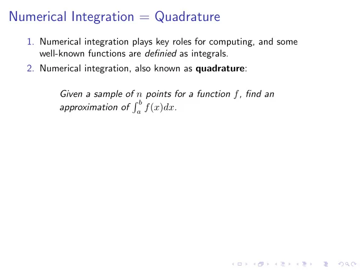
Numerical Integration = Quadrature 1. Numerical integration plays key roles for computing, and some well-known functions are definied as integrals. 2. Numerical integration, also known as quadrature : Given a sample of n points for a function f , find an � b approximation of a f ( x ) dx .

Numerical Integration = Quadrature Interpolatory quadrature, also known as Newton-Cotes rules let n � f ( x ) = a i φ i ( x ) i =1 where φ i ( x ) are basis functions (see Chapter 13 on Interpolation). Then the integral of f : � b �� b n � � f ( x ) = a i φ i ( x ) a a i =1

Numerical Integration = Quadrature Newton-Cotes rules: ◮ n = 1 , midpoint rule error = O (( b − a ) 3 ) ◮ n = 1 , trapezoidal rule error = O (( b − a ) 3 ) Note: the same order as the midpoint rule ◮ n = 2 , Simpson’s rule error = O (( b − a ) 5 )

Numerical Integration = Quadrature Composite rules : Let [ a, b ] be subdivided into k intervals, say, take ∆x = b − a k , and x i = a + ( i − 1) ∆x . ◮ the composite trapezoidal rule is given by � b k � f ( x i ) + f ( x i +1 ) � � f ( x ) ≈ ∆x 2 a i =1 � 1 2 f ( a ) + f ( x 2 ) + · · · + f ( x k ) + 1 � = 2 f ( b ) ∆x error = O (( ∆x ) 3 ) × b − a ∆x = O (( ∆x ) 2 ) . ◮ By a similar scheme, we can also derive a composite Simpson’s rule. error = O ( ∆x 5 ) × b − a ∆x = O ( ∆x 4 ) .

Numerical Integration = Quadrature Adaptive Simpson’s quadrature � b ◮ Goal : approx. I = a f ( x ) dx to within an error tolerance ǫ > 0 . ◮ step 1: Simpson’s rule with h = ( b − a ) / 2 I = S ( a, b ) − E 1 := S 1 − E 1 ◮ step 2: Composite Simpson’s rule with h 1 = ( b − a ) / 2 2 I = S ( a, a + b ) + S ( a + b , b ) − E 2 := S 2 − E 2 2 2 ◮ It can be shown that E 1 ≈ 16 E 2 . Then S 1 − S 2 = E 1 − E 2 ≈ 15 E 2 . which implies that | I − S 2 | = | E 2 | ≈ 1 15 | S 1 − S 2 | .

Numerical Integration = Quadrature Adaptive Simpson’s quadrature, cont’d ◮ If | S 1 − S 2 | / 15 < ǫ , then | I − S 2 | < ǫ . S 2 is sufficiently accuracy. ◮ Otherwise, apply the same error estimation procedure to the subintervals [ a, a + b 2 ] and [ a + b 2 , b ] , respectively to determine if the approximation to the integral on each subinterval is within a tolerance of ǫ/ 2 ◮ Recursive algorithm ◮ MATLAB code: quadtx.m

Numerical Integration = Quadrature 1. Quadrature rules in a general form � b n � f ( x ) dx ≈ Q ( f ) = w i f ( x i ) a i =1 where x i are knots , and w i are weights . 2. The choices of { x i } and { w i } determine a quadrature rule. 3. The method of undetermined coefficients fix { x i } , choose { w i } so that Q ( f ) approximate the integral of f for reasonably smooth functions.

Numerical Integration = Quadrature Example of the method of undetermined coefficients ◮ Let x 1 = 0 , x 2 = 1 / 2 and x 3 = 1 . pick f 1 ( x ) = 1 , f 2 ( x ) = x and f 3 ( x ) = x 2 such that � 1 f 1 ( x ) dx = w 1 f 1 ( x 1 ) + w 2 f 1 ( x 2 ) + w 3 f 1 ( x 3 ) 0 � 1 f 2 ( x ) dx = w 1 f 2 ( x 1 ) + w 2 f 2 ( x 2 ) + w 3 f 2 ( x 3 ) 0 � 1 f 3 ( x ) dx = w 1 f 3 ( x 1 ) + w 2 f 3 ( x 2 ) + w 3 f 3 ( x 3 ) 0 ◮ Consequently, we have the Simplson’s rule � 1 f ( x ) dx ≈ Q ( f ) = 1 6 f (0) + 2 3 f (1 2) + 1 6 f (1) 0 ◮ By the change of interval [ a, b ] → [0 , 1] , x = a + ( b − a ) y , we have the Simplson’s rule on the interval [ a, b ] : � b � 1 � 6 f ( a ) + 2 3 f ( b + a ) + 1 f ( x ) dx ≈ Q ( f ) = ( b − a ) 6 f ( b ) 2 a