Numerical Integration Numerical Integration 1 / 11 Objective b - - PowerPoint PPT Presentation

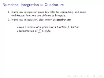
Numerical Integration

Numerical Integration 1 / 11

Objective

Approximate b

a

f (x) dx

Numerical Integration 2 / 11

Objective

Approximate b

a

f (x) dx A jog down Calc I/II lane The integral is the area under the curve, i.e between the curve and x-axis

Numerical Integration 2 / 11

Objective

Approximate b

a

f (x) dx A jog down Calc I/II lane The integral is the area under the curve, i.e between the curve and x-axis However, analytical anti-derivatives are not always easy to write down, making evaluation of some basic definite integrals difficult. b

a

ex2 dx

Numerical Integration 2 / 11

Objective

Approximate b

a

f (x) dx A jog down Calc I/II lane The integral is the area under the curve, i.e between the curve and x-axis However, analytical anti-derivatives are not always easy to write down, making evaluation of some basic definite integrals difficult. b

a

ex2 dx In some practical cases, we do not have an analytical representation

• f f but we still want to approximate the integral

Numerical Integration 2 / 11

Objective

Approximate b

a

f (x) dx A jog down Calc I/II lane The integral is the area under the curve, i.e between the curve and x-axis However, analytical anti-derivatives are not always easy to write down, making evaluation of some basic definite integrals difficult. b

a

ex2 dx In some practical cases, we do not have an analytical representation

• f f but we still want to approximate the integral

Numerical integration techniques are necessary to approximate the integral

Numerical Integration 2 / 11

Approximating b

a

f (x) dx (basic idea)

Approximate the “area” under the curve on [a, b] using simple sub-regions

Numerical Integration 3 / 11

Approximating b

a

f (x) dx (basic idea)

Approximate the “area” under the curve on [a, b] using simple sub-regions

Sub-divide the interval [a, b] into n subintervals of equal width ∆x = b − a n

Numerical Integration 3 / 11

Approximating b

a

f (x) dx (basic idea)

Approximate the “area” under the curve on [a, b] using simple sub-regions

Sub-divide the interval [a, b] into n subintervals of equal width ∆x = b − a n More sophisticated methods use adaptive widths of subinterval depending on the behavior of the function

Numerical Integration 3 / 11

Approximating b

a

f (x) dx (basic idea)

Approximate the “area” under the curve on [a, b] using simple sub-regions

Sub-divide the interval [a, b] into n subintervals of equal width ∆x = b − a n More sophisticated methods use adaptive widths of subinterval depending on the behavior of the function As the number of sub-intervals increases, we obtain a more accurate approximation of the area under the curve

Desmos demo Numerical Integration 3 / 11

Approximating b

a

f (x) dx (Implementation)

Rectangles

1 Divide [a, b] so that

a = x1 < x2 < · · · < xn < xn+1 = b, k = 1, 2, . . . , n with xk = a + (k − 1)∆x

Numerical Integration 4 / 11

Approximating b

a

f (x) dx (Implementation)

Rectangles

1 Divide [a, b] so that

a = x1 < x2 < · · · < xn < xn+1 = b, k = 1, 2, . . . , n with xk = a + (k − 1)∆x

2 On each sub-interval [xk, xk+1] select a sample point, x∗

k ∈ [xk, xk+1]

Numerical Integration 4 / 11

Approximating b

a

f (x) dx (Implementation)

Rectangles

1 Divide [a, b] so that

a = x1 < x2 < · · · < xn < xn+1 = b, k = 1, 2, . . . , n with xk = a + (k − 1)∆x

2 On each sub-interval [xk, xk+1] select a sample point, x∗

k ∈ [xk, xk+1]

3 Define the height of each sub-rectangle as f (x∗

k) so that the area of

each sub-rectangle is f (x∗)∆x

4 Summing up for the n sub-intervals

b

a

f (x) dx ≈

n

• k=1

f (x∗

k)∆x

Numerical Integration 4 / 11

Approximating b

a

f (x) dx (Implementation)

Trapeziods

1 Each trapezoid has a base of [xk, xk+1] with parallel sides of length

f (xk) and f (xk+1)

Numerical Integration 5 / 11

Approximating b

a

f (x) dx (Implementation)

Trapeziods

1 Each trapezoid has a base of [xk, xk+1] with parallel sides of length

f (xk) and f (xk+1)

2 The area of the k-th Trapezoid is

∆x 2

• f (xk) + f (xk+1)
• Numerical Integration

5 / 11

Approximating b

a

f (x) dx (Implementation)

Trapeziods

1 Each trapezoid has a base of [xk, xk+1] with parallel sides of length

f (xk) and f (xk+1)

2 The area of the k-th Trapezoid is

∆x 2

• f (xk) + f (xk+1)
• 3 Summing up for the n sub-intervals

b

a

f (x) dx ≈ ∆x 2

n

• k=1
• f (xk) + f (xk+1)
• Numerical Integration

5 / 11

Approximating b

a

f (x) dx (Implementation)

Trapezoids

b

a

f (x) dx ≈ ∆x 2

n

• k=1
• f (xk) + f (xk+1)
• = ∆x

2

• [f (x1) + f (x2)] + [(f (x2) + f (x3)] + · · · + [f (xn−1) + f (xn)] + [f (xn) + f (xn+1)]
• = ∆x

2

• f (x1) + 2f (x2) + · · · + 2f (xn) + f (xn+1)
• b

a

f (x) dx = ∆x 2

• f (x1) + 2

n

• k=2

f (xk) + f (xn+1)

• Numerical Integration

6 / 11

Error Analysis (MA 428)

Theorem Assuming max

a≤x≤b |f ′′(x)| ≤ M. Then the midpoint method has error

M(b − a)(∆x)2 24 and the Trapezoidal method has error M(b − a)(∆x)2 12

Numerical Integration 7 / 11

Simpson’s Method for approximating b

a

f (x) dx

Approximate the area under the function using second order curves

Numerical Integration 8 / 11

Simpson’s Method for approximating b

a

f (x) dx

Approximate the area under the function using second order curves

1

Divide [a, b] into n sub-intervals of width ∆x = b−a

n , where n is even.

Numerical Integration 8 / 11

Simpson’s Method for approximating b

a

f (x) dx

Approximate the area under the function using second order curves

1

Divide [a, b] into n sub-intervals of width ∆x = b−a

n , where n is even.

2

On each pair of sub-intervals [xk−1, xk] and [xk, xk+1] (k = 2, · · · , n) approximate the area under the curve with a quadratic function passing through the points:

• xk−1, f (xk−1)
• ,
• xk, f (xk)
• and (xk+1, f (xk+1))

Numerical Integration 8 / 11

Simpson’s Method for approximating b

a

f (x) dx

Approximate the area under the function using second order curves

1

Divide [a, b] into n sub-intervals of width ∆x = b−a

n , where n is even.

2

On each pair of sub-intervals [xk−1, xk] and [xk, xk+1] (k = 2, · · · , n) approximate the area under the curve with a quadratic function passing through the points:

• xk−1, f (xk−1)
• ,
• xk, f (xk)
• and (xk+1, f (xk+1))

3

The area under each parabola on [xk−1, xk] and [xk, xk+1] is ∆x 3

• f (xk−1) + 4f (xk) + f (xk+1)
• Numerical Integration

8 / 11

Simpson’s Method for approximating b

a

f (x) dx

Approximate the area under the function using second order curves

1

Divide [a, b] into n sub-intervals of width ∆x = b−a

n , where n is even.

2

On each pair of sub-intervals [xk−1, xk] and [xk, xk+1] (k = 2, · · · , n) approximate the area under the curve with a quadratic function passing through the points:

• xk−1, f (xk−1)
• ,
• xk, f (xk)
• and (xk+1, f (xk+1))

3

The area under each parabola on [xk−1, xk] and [xk, xk+1] is ∆x 3

• f (xk−1) + 4f (xk) + f (xk+1)
• 4

Summing up over all sub-intervals b

a

f (x) dx ≈ ∆x 3

• f1 + 4f2 + 2f3 + 4f4 + · · · + 2fn−1 + 4fn + fn+1
• Numerical Integration

8 / 11

Error Analysis (MA 428)

Theorem Assuming max

a≤x≤b |f (4)(x)| ≤ M. Then the Simpson’s method has error

M(b − a)(∆x)4 180 Composite Simpson’s method has a convergence rate of O(∆x)4 compared to Midpoint and Trapezoidal that are O(∆x)2.

Numerical Integration 9 / 11

Error comparison

log10(∆x)

• 4
• 3.5
• 3
• 2.5
• 2
• 1.5
• 1

log10(error)

• 16
• 14
• 12
• 10
• 8
• 6
• 4
• 2

Comparison

Simpsons Midpoint Trapeziod

Midpoint and Trapezoidal methods are second order in ∆x i.e. O((∆x)2) Simpsons method is fourth order in ∆x i.e. O((∆x)4)

Numerical Integration 10 / 11

Generalized formula

Higher order methods of the form b

a

f (x) dx =

N

• i=1

f (xi)wi These methods can be extended to 2D and 3D integrals (see MA 428).

Numerical Integration 11 / 11