Lecture 17 : Double Integrals 0/ 15 Some of you have not learned - PDF document

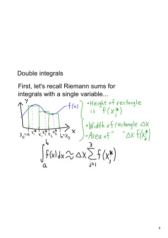
Lecture 17 : Double Integrals 0/ 15

Some of you have not learned how to do double integrals. In this course you will need to do double integrals over rectangles and I will now explain how to do such calculations. Partial (Indefinite) Integration � In one variable calculus you learned about the indefinite integral f ( x ) dx . The point of the indefinite integral was that it was an inverse of the derivative �� � d f ( x ) dx = f ( x ) dx (In fact this is the definition of the) indefinite integral. 1/ 15 Lecture 17 : Double Integrals

So x 3 dx = x 4 � 4 and x 4 d 4 = x 3 dx The indefinite integral is defined only up to an arbitrary constant, “the constant of integration”. The fundamental theorem of calculus then says that to evaluate the definite b � f ( x ) dx you take any indefinite integral, evaluate it at the upper limit b integral 0 and at the lower limit a and subtract the latter from the former. 2/ 15 Lecture 17 : Double Integrals

Now in two variable calculus you have two “partial” derivatives ∂ f ∂ x ( x , y ) and ∂ f � � ∂ y ( x , y ) so you have two partial indefinite integrals f ( x , y ) dx and f ( x , y ) dy . So (by definition) �� � ∂ f ( x , y ) dx = f ( x , y ) ∂ x �� � ∂ f ( x , y ) dy = f ( x , y ) . ∂ y Let’s compute � ( x 2 + y 2 ) dx . The idea is to tract y as a constant. 3/ 15 Lecture 17 : Double Integrals

The partial indefinite integral in x is defined only up to a function of y. (because ∂ ∂ x g ( y ) = 0). Let’s do a harder one � sin xy dy = − 1 x cos xy . (check chain rule 4/ 15 Lecture 17 : Double Integrals

Partial (Definite) Integrals Once you have the partial indefinite integral you have the partial definite integral 2 � x 3 � � � x = 2 ( x 2 + y 2 ) dx = 3 + y 3 x � � � x = 1 1 � 8 � � 1 � 3 + 2 y 2 3 + y 2 = − = y 2 + 7 3 The Golden Rule Treat y as a constant throughout and do the one variable integral with respect to x . Note the output is a function of y. 5/ 15 Lecture 17 : Double Integrals

Using Partial Integration to Evaluate Double Integrals over Rectangles Just as we use the indefinite integral in one variable to evaluate definite integrals in one variable we will use the partial integrals to evaluate (definite) double integrals (*) The notation is very confusing because of tradition. Here the x -limits are a and b and the y -limits are c and d so a and b go with dx and c and d go with dy. Watch out for this later. 6/ 15 Lecture 17 : Double Integrals

So we have a rectangle R [ a , b ] × [ c , d ] in the xy -plane When you learn integration theory correctly you will write this integral as � � f ( x , y ) dx dy (**) R However putting in the limits a , b and c , d is helpful for computations. Think of rewriting (**) as x = b y = d � � f ( x , y ) dx dy . x = a y = c 7/ 15 Lecture 17 : Double Integrals

So how do you compute 2 1 � � ( x 2 + y 2 ) dx dy (**) 1 0 So the rectangle R is a square 1 0 1 2 Here is how you compute (**). There are two ways. It is a famous theorem of Fubini that they lead to the same result. We will see this in our example. Pick the way that leads to the easiest computations. 8/ 15 Lecture 17 : Double Integrals

First way (do the x -integration first) 1 Write (**) as Z Remember 1 and 2 go with dx and 0 and 1 go with dy (see page 6) 2 Do the inside partial definite integral. The output will be the function of y g ( y ) = y 2 + 7 3 (from page 5). 9/ 15 Lecture 17 : Double Integrals

3 Do a one variable definite integral of g ( y ) with respect to y from 0 to 1. 1 y = 0 � y 3 �� � � � y 2 + 7 3 + 7 � dy = � 3 y � 3 � � y = 0 0 = 1 3 + 7 3 = 8 3 That’s it. The above method is said to evaluate the double integral by iterated one variable integrals. However the first step is new it is a partial integral with respect to x. 10/ 15 Lecture 17 : Double Integrals

Second way (do the y -integration first) 1 This time we write (**) as 2 Now we do the partial integration with respect to y so x is a constant. 1 y = 1 x 2 y + y 3 �� � � ( x 2 + y 2 ) dy = � � � 3 � � y = 0 0 = x 2 + 1 3 The output is a function of x . 11/ 15 Lecture 17 : Double Integrals

3 Perform the one variable integration of the output function h ( x ) = x 2 + 1 3 with respect to x . 2 x = 2 �� � x 3 � � � x 2 + 1 3 + x � dx = � � 3 3 � � x = 1 1 � 8 � � 1 � 3 + 2 3 + 1 = − 3 3 = 8 3 So as predicted we got the same answer no matter which order we chose to perform the iterated integrals. 12/ 15 Lecture 17 : Double Integrals

Double Integrals of Product Functions over Rectangles There is one case in which double integrals one particularly easy to compute. Definition Let f ( x , y ) be a function of two variables x and y. The f ( x , y ) is a product function if there exist g ( x ) and h ( g ) such that f ( x , y ) = g ( x ) h ( y ) 13/ 15 Lecture 17 : Double Integrals

Examples f ( x , y ) = e x sin y YES (it is a product) f ( x , y ) = e x + sin y NO (it is not a product) f ( x , y ) = xy YES f ( x , y ) = x + y NO Theorem b d � � ( g ( x ) h ( y )) dx dy a c b d     � �          g ( x ) dx   h ( y ) dy                          a c Z Most functions of x and y are NOT product functions. 14/ 15 Lecture 17 : Double Integrals

Theorem (Cont.) So 1 1 1 1     � � � �         ( xy 2 ) dx dy = g 2 dy     x dx                         0 0 0 0 � 1 � � 1 � = 1 = 2 3 6 So a double integral of a product function over a rectangle is the product of two one variable integrals (one in x, the other in y). 15/ 15 Lecture 17 : Double Integrals