Reduced order modelling in multi-parametrized system: applications - PowerPoint PPT Presentation
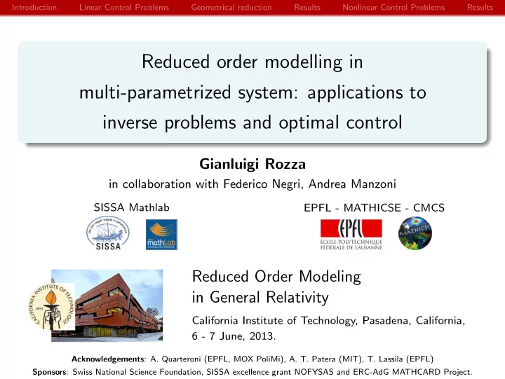
Introduction Linear Control Problems Geometrical reduction Results Nonlinear Control Problems Results Reduced order modelling in multi-parametrized system: applications to inverse problems and optimal control Gianluigi Rozza in
Introduction Linear Control Problems Geometrical reduction Results Nonlinear Control Problems Results Reduced order modelling in multi-parametrized system: applications to inverse problems and optimal control Gianluigi Rozza in collaboration with Federico Negri, Andrea Manzoni SISSA Mathlab EPFL - MATHICSE - CMCS Reduced Order Modeling in General Relativity California Institute of Technology, Pasadena, California, 6 - 7 June, 2013. Acknowledgements : A. Quarteroni (EPFL, MOX PoliMi), A. T. Patera (MIT), T. Lassila (EPFL) Sponsors : Swiss National Science Foundation, SISSA excellence grant NOFYSAS and ERC-AdG MATHCARD Project.
Introduction Linear Control Problems Geometrical reduction Results Nonlinear Control Problems Results Outline 1. Introduction Motivation and ingredients 2. Parametrized linear-quadratic Optimization Problems Saddle-point formulation Reduced Basis (RB) methodology for computational reduction 3. Geometrical parametrization 4. Applications and results Optimal control of a Graetz advection-diffusion problem (L0) Application to a surface reconstruction problem in haemodynamics (L1) Stokes constraint: a numerical test (L2) and a data assimilation problem for blood flows (L3) 5. Parametrized nonlinear control problems for the Navier-Stokes equations Newton-SQP method – analogies with the linear case Brezzi-Rappaz-Raviart theory to obtain error bounds Benchmark test: vorticity minimization (NL1)
Introduction Linear Control Problems Geometrical reduction Results Nonlinear Control Problems Results Complex parametrized systems ∂ v ∂ t − ν ∆ v + ( v · ∇ ) v + ∇ π = f in Ω( µ ) Parametrized Simulation div v = 0 in Ω( µ ) Problems ∂ C ∂ t − ∇ · ( µ c ∇ C ) + v · ∇ C = 0 in Ω( µ ) min J ( y , u ; µ ) = F ( y ; µ ) + G ( u ; µ ) Parametrized Data assimilation and subject to Inverse Problems − ν ( µ )∆ y + b ( µ ) · ∇ y = 0 in Ω( µ ) y = u on Γ( µ ) min J ( v , π, u ; µ ) = F ( v , π ; µ ) + G ( u ; µ ) subject to Parametrized Optimization − ν ∆ v + ( v · ∇ ) v + ∇ π = 0 in Ω( µ ) Problems div v = 0 in Ω( µ ) v = u on Γ D ( µ )
Introduction Linear Control Problems Geometrical reduction Results Nonlinear Control Problems Results Complexity in haemodynamics The main obstacle to make mathematical models extensively useful and reliable in the clinical context is that they have to be personalized Many quantities required by the numerical simulations cannot be always obtained through direct measurements and thus need to be estimated using the available clinical measurements The ultimate goal would be to optimize the therapeutic intervention depending on the patient attributes
Introduction Linear Control Problems Geometrical reduction Results Nonlinear Control Problems Results Complexity in haemodynamics Parametrized Simulation Problems Many quantities required by the numerical simulations cannot be always obtained through direct measurements and thus need to be estimated using the available clinical measurements The ultimate goal would be to optimize the therapeutic intervention depending on the patient attributes
Introduction Linear Control Problems Geometrical reduction Results Nonlinear Control Problems Results Complexity in haemodynamics Parametrized Simulation Problems Parametrized Data assimilation and Inverse Problems The ultimate goal would be to optimize the therapeutic intervention depending on the patient attributes
Introduction Linear Control Problems Geometrical reduction Results Nonlinear Control Problems Results Complexity in haemodynamics Parametrized Simulation Problems Parametrized Data assimilation and Inverse Problems Parametrized Optimization Problems
Introduction Linear Control Problems Geometrical reduction Results Nonlinear Control Problems Results Models and problems surface reconstruction of blood flow profiles inverse problems: reconstruction of boundary conditions by experimental measures/observations flow control: vorticity reduction by suction/injection of fluid through the boundary Steady state system : advection-diffusion, Stokes or Navier-Stokes equations Control variables : distributed in the domain or along the boundary Parameters : they can be physical/geometrical quantities describing the state system or related to observation measurements in the cost functional
Introduction Linear Control Problems Geometrical reduction Results Nonlinear Control Problems Results Optimal control problems [Lions, 1971] In general, an optimal control problem (OCP) consists of: a control function u , which can be seen as an input for the system, y ( u ) u STATE a controlled system, i.e. an Output J ( y , u ) PROBLEM input-output process: E ( y , u ) = 0, being y the state variable Optimization: an objective functional to be update control u minimized: J ( y , u )
Introduction Linear Control Problems Geometrical reduction Results Nonlinear Control Problems Results Optimal control problems [Lions, 1971] In general, an optimal control problem (OCP) consists of: a control function u , which can be seen as an input for the system, y ( u ) u STATE a controlled system, i.e. an Output J ( y , u ) PROBLEM input-output process: E ( y , u ) = 0, being y the state variable Optimization: an objective functional to be update control u minimized: J ( y , u ) find the optimal control u ∗ and the state y ( u ∗ ) such that the cost functional ( OCP ) J ( y , u ) is minimized subject to E ( y , u ) = 0
Introduction Linear Control Problems Geometrical reduction Results Nonlinear Control Problems Results Optimal control problems [Lions, 1971] In general, an optimal control problem (OCP) consists of: a control function u , which can be seen as an input for the system, y ( u ) u STATE a controlled system, i.e. an Output J ( y , u ) PROBLEM input-output process: E ( y , u ) = 0, being y the state variable Optimization: an objective functional to be update control u minimized: J ( y , u ) find the optimal control u ∗ and the state y ( u ∗ ) such that the cost functional ( OCP ) J ( y , u ) is minimized subject to E ( y , u ) = 0 We restrict attention to: 2 � y − y d � 2 + α quadratic cost functionals, e.g. J ( y , u ) = 1 2 � u � 2
Introduction Linear Control Problems Geometrical reduction Results Nonlinear Control Problems Results Parametrized optimal control problems A parametrized optimal control problem (OCP µ ) consists of: y d ( µ ) (data) a control function u ( µ ), which can µ be seen as an input for the system, u ( µ ) y ( u ( µ )) STATE a controlled system, i.e. an Output J ( y , u ; µ ) PROBLEM input-output process: E ( y ( µ ) , u ( µ ); µ ) = 0, Optimization: an objective functional to be update control u minimized: J ( y ( µ ) , u ( µ ); µ ) given µ ∈ D , find the optimal control u ∗ ( µ ) and the state y ∗ ( µ ) such that the ( OCP µ ) cost functional J ( y ( µ ) , u ( µ ); µ ) is minimized subject to E ( y ( µ ) , u ( µ ); µ ) = 0 where µ ∈ D ⊂ R p denotes a p -vector whose components can represent: coefficients in boundary conditions physical parametrization geometrical configurations data (observation)
Introduction Linear Control Problems Geometrical reduction Results Nonlinear Control Problems Results Reduction strategies for Parametrized Optimal Control Problems y d ( µ ) (data) µ PROBLEM : given µ ∈ D ⊂ R p , u ( µ ) y ( u ( µ )) STATE Output J ( y , u ; µ ) PROBLEM E min J ( y , u ; µ ) y , u s.t. E ( y , u ; µ ) = 0 Optimization: update control u The computational effort may be unacceptably high and, often, unaffordable when performing the optimization process for many different parameter values ( many-query context) for a given new configuration, we want to compute the solution in a rapid way ( real-time context) Goal : to achieve the accuracy and reliability of a high fidelity approximation but at greatly reduced cost of a low order model
Introduction Linear Control Problems Geometrical reduction Results Nonlinear Control Problems Results Parametrized control problems vs Parametric Control min J ( y , u ; µ ) = F ( y ; µ ) + G ( u ; µ ) min J ( v , π, u ; µ ) = F ( v , π ; µ ) + G ( u ; µ ) subject to subject to − ν ( µ )∆ y + b ( µ ) · ∇ y = u in Ω( µ ) − ν ∆ v + ( v · ∇ ) v + ∇ π = 0 in Ω( µ ) y = g on Γ D ( µ ) div v = 0 in Ω( µ ) − ν ( µ ) ∇ y · n = 0 on Γ N ( µ ) v = u on Γ D ( µ ) Control variables : distributed in the domain or along the boundary In many previous works the idea was to reduce the complexity of the problem by introducing a Parametric Control , e.g. u ( µ c ) = � µ c i h i ( x ) We need to introduce further parameters [ µ , µ c ] How many terms to obtain good approximation of the control space? Certification of the optimum still missing (need reduced model of the adjoint) A priori constraints on the range of variations of the parameters µ c
Recommend
More recommend
Explore More Topics
Stay informed with curated content and fresh updates.
