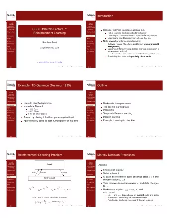
Reinforcement Learning Steve Tanimoto University of California, - PowerPoint PPT Presentation

Feb 05, 2024 •175 likes •311 views

Reinforcement Learning Steve Tanimoto University of California, Berkeley [These slides were created by Dan Klein and Pieter Abbeel for CS188 Intro to AI at UC Berkeley. All CS188 materials are available at http://ai.berkeley.edu.] Reinforcement

Reinforcement Learning Steve Tanimoto University of California, Berkeley [These slides were created by Dan Klein and Pieter Abbeel for CS188 Intro to AI at UC Berkeley. All CS188 materials are available at http://ai.berkeley.edu.]
Reinforcement Learning
Reinforcement Learning Agent State: s Actions: a Reward: r Environment  Basic idea:  Receive feedback in the form of rewards  Agent’s utility is defined by the reward function  Must (learn to) act so as to maximize expected rewards  All learning is based on observed samples of outcomes!
Example: Learning to Walk Initial A Learning Trial After Learning [1K Trials] [Kohl and Stone, ICRA 2004]
Example: Toddler Robot [Tedrake, Zhang and Seung, 2005] [Video: TODDLER – 40s]
Active Reinforcement Learning
Active Reinforcement Learning  Full reinforcement learning: optimal policies (like value iteration)  You don’t know the transitions T(s,a,s’)  You don’t know the rewards R(s,a,s’)  You choose the actions now  Goal: learn the optimal policy / values  In this case:  Learner makes choices!  Fundamental tradeoff: exploration vs. exploitation  This is NOT offline planning! You actually take actions in the world and find out what happens…
Detour: Q-Value Iteration  Value iteration: find successive (depth-limited) values  Start with V 0 (s) = 0, which we know is right  Given V k , calculate the depth k+1 values for all states:  But Q-values are more useful, so compute them instead  Start with Q 0 (s,a) = 0, which we know is right  Given Q k , calculate the depth k+1 q-values for all q-states:
Q-Learning  Q-Learning: sample-based Q-value iteration  Learn Q(s,a) values as you go  Receive a sample (s,a,s’,r)  Consider your old estimate:  Consider your new sample estimate:  Incorporate the new estimate into a running average: [Demo: Q-learning – gridworld (L10D2)] [Demo: Q-learning – crawler (L10D3)]
Video of Demo Q-Learning -- Gridworld
Video of Demo Q-Learning -- Crawler
Q-Learning Properties  Amazing result: Q-learning converges to optimal policy -- even if you’re acting suboptimally!  This is called off-policy learning  Caveats:  You have to explore enough  You have to eventually make the learning rate small enough  … but not decrease it too quickly  Basically, in the limit, it doesn’t matter how you select actions (!)

Recommend

Reinforcement Learning AIMA Chapters: 21.1, 21.2, 21.3. Sutton and Barto, Reinforcement Learning:

Reinforcement Learning Reinforcement Learning AIMA Chapters: 21.1, 21.2, 21.3. Sutton and Barto, Reinforcement Learning: an Introduction, 2nd Edition: Chapters 6 (6.1 6.5) Outline Reinforcement Learning Reinforcement Learning: the

589 views • 27 slides

Reinforcement Learning Timothy Chou Charlie Tong Vincent Zhuang April 19, 2016 Reinforcement

Reinforcement Learning Q-Learning Deep Q-Learning on Atari Reinforcement Learning Timothy Chou Charlie Tong Vincent Zhuang April 19, 2016 Reinforcement Learning Q-Learning Deep Q-Learning on Atari Table of Contents Reinforcement Learning

939 views • 63 slides

RL Overview of topics About Reinforcement Learning The Reinforcement Learning Problem

Introduction to Reinforcement Learning RL Overview of topics About Reinforcement Learning The Reinforcement Learning Problem Inside an RL agent Temporal difference learning Many faces of Reinforcement Learning What is

552 views • 35 slides

Reinforcement Learning UMaine COS 470/570 Introduction to AI Why reinforcement learning?

Reinforcement Learning<br/><br/> 4/25/19, 8*06 PM Reinforcement Learning<br/><br/> 4/25/19, 8*06 PM Reinforcement Learning UMaine COS 470/570 Introduction to AI Why reinforcement learning? Spring 2019 Created:

372 views • 15 slides

Reinforcement Learning and Simulation-Based Search David Silver Reinforcement Learning and

Reinforcement Learning and Simulation-Based Search Reinforcement Learning and Simulation-Based Search David Silver Reinforcement Learning and Simulation-Based Search Outline 1 Reinforcement Learning 2 Simulation-Based Search 3 Planning Under

425 views • 20 slides

Reinforcement Learning Reinforcement Learning Reinforcement Learning in a nutshell g Imagine

Reinforcement Learning Reinforcement Learning Reinforcement Learning in a nutshell g Imagine playing a new game whose rules you dont know; after a hundred or so moves your don t know; after a hundred or so moves, your opponent announces, You

512 views • 30 slides

Safe Reinforcement Learning Philip S. Thomas Stanford CS234: Reinforcement Learning, Guest

Safe Reinforcement Learning Philip S. Thomas Stanford CS234: Reinforcement Learning, Guest Lecture May 24, 2017 Lecture overview What makes a reinforcement learning algorithm safe ? Notation Creating a safe reinforcement learning

1.43k views • 88 slides

CS885 Reinforcement Learning Module 2: June 6, 2020 Maximum Entropy Reinforcement Learning

CS885 Reinforcement Learning Module 2: June 6, 2020 Maximum Entropy Reinforcement Learning Haarnoja, Tang et al. (2017) Reinforcement Learning with Deep Energy Based Policies, ICML . Haarnoja, Zhou et al. (2018) Soft Actor-Critic: Off-Policy

684 views • 24 slides

Introduction to Reinforcement Learning Kevin Chen and Zack Khan Lecture 1: Introduction to

Lecture 1: Introduction to Reinforcement Learning Introduction to Reinforcement Learning Kevin Chen and Zack Khan Lecture 1: Introduction to Reinforcement Learning Outline 1. Course Logistics 2. What is Reinforcement Learning? 3.

930 views • 67 slides

Introduction to Reinforcement Learning and Q-Learning Skyler Seto (ss3349) May 2, 2016 Skyler

Reinforcement Learning and Markov Decision Process Q-Learning Q-Learning Convergence Introduction to Reinforcement Learning and Q-Learning Skyler Seto (ss3349) May 2, 2016 Skyler Seto (ss3349) Introduction to Reinforcement Learning and

565 views • 27 slides

7. Motor Control and Reinforcement Learning Outline A. Action Selection and Reinforcement B.

7. Motor Control and Reinforcement Learning Outline A. Action Selection and Reinforcement B. Temporal Difference Reinforcement Learning C. PVLV Model D. Cerebellum and Error-driven Learning 2/23/18 COSC 494/594 CCN 2 Sensory-Motor Loop

791 views • 56 slides

1 Deep Reinforcement Learning Qianqian Li, Nayeon Koong, Langtian He What is deep reinforcement

1 Deep Reinforcement Learning Qianqian Li, Nayeon Koong, Langtian He What is deep reinforcement learning? Agent/Actor + Action + Environment + State + Reward How does reinforcement learning work?

793 views • 31 slides

Introduction CSCE CSCE 496/896 496/896 Lecture 7: Lecture 7: Reinforcement Reinforcement

Introduction CSCE CSCE 496/896 496/896 Lecture 7: Lecture 7: Reinforcement Reinforcement CSCE 496/896 Lecture 7: Learning Learning Consider learning to choose actions, e.g., Stephen Scott Reinforcement Learning Stephen Scott Robot

434 views • 9 slides

Path following with reinforcement learning for autonomous cars - Mozzam Motiwala (IAS) Index

Path following with reinforcement learning for autonomous cars - Mozzam Motiwala (IAS) Index Basics of Reinforcement Learning Model Based vs Model Free Reinforcement Learning Autonomous Car collision avoidance What is Reinforcement

714 views • 24 slides

CSC2621 Topics in Robotics Reinforcement Learning in Robotics Week 11: Hierarchical Reinforcement

CSC2621 Topics in Robotics Reinforcement Learning in Robotics Week 11: Hierarchical Reinforcement Learning Animesh Garg Between MDPs and semi-MDPs: A framework for temporal abstraction in reinforcement learning Richard S. Sutton , Doina

2.19k views • 29 slides

Machine Learning for NLP Reinforcement learning Aurlie Herbelot 2019 Centre for Mind/Brain

Machine Learning for NLP Reinforcement learning Aurlie Herbelot 2019 Centre for Mind/Brain Sciences University of Trento 1 Introduction 2 Reinforcement learning: intuition Reinforcement learning: like learning to ride a bicycle.

1.18k views • 58 slides

t t rt t

t t rt t r rs rs r ss st

644 views • 38 slides

ABB: writing the future of industries in a changing world 2 nd industrial revolution 4 th

ABB: writing the future of industries in a changing world 2 nd industrial revolution 4 th industrial revolution 3 rd industrial revolution (19 th century) (20 th century) (21 st century) + Electrification + Industrial automation +

325 views • 5 slides

In-Place (Bijective) BWT Transforms Dominik Kppl Kyushu University Daiki Hashimoto Tohoku

In-Place (Bijective) BWT Transforms Dominik Kppl Kyushu University Daiki Hashimoto Tohoku University Diptarama Ayumi Shinohara data structures Burrows-Wheeler Transform (BWT) [Burrows,Wheeler '94] Bijective BWT (BBWT) [Gil,Scott '12]

905 views • 88 slides

Computational Linguistics II: Parsing Overview, Left-Recursion, Bottom-up Parsing Frank Richter

Computational Linguistics II: Parsing Overview, Left-Recursion, Bottom-up Parsing Frank Richter & Jan-Philipp S ohn fr@sfs.uni-tuebingen.de, jp.soehn@uni-tuebingen.de Computational Linguistics II: Parsing p.1 The Big Picture

667 views • 43 slides

Utilize Partially Faulty Links in Networks-on-Chip Changlin Chen, Ye Lu , Sorin D. Cotofana

A Novel Flit Serialization Strategy to Utilize Partially Faulty Links in Networks-on-Chip Changlin Chen*, Ye Lu , Sorin D. Cotofana* ECIT, QUB *Computer engineering, TU Delft {c.chen-2, S.D.Cotofana}@tudelft.nl ylu10@qub.ac.uk NOCS 2012

468 views • 20 slides

Distinguishing strings From lecture 3: Definition Let L be language over , and let x , y

Distinguishing strings From lecture 3: Definition Let L be language over , and let x , y . Then x , y are distinguishable wrt L ( L-distinguishable ), if there exists z with xz L and yz / L or xz / L and yz

450 views • 19 slides

Learning Regular Sets Author: Dana Angluin Presented by: M. Andre na Francisco Department

Learning Regular Sets Author: Dana Angluin Presented by: M. Andre na Francisco Department of Computer Science Uppsala University February 3, 2014 Minimally Adequate Teachers A Minimally Adequate Teacher (MAT) is an Oracle that must

717 views • 33 slides

Efficient algorithms for two extensions of LPF table: the power of suffix arrays M.Crochemore

Efficient algorithms for two extensions of LPF table: the power of suffix arrays M.Crochemore C.S.Iliopoulos M.Kubica W.Rytter T.Wale SOFSEM 2010 M.Crochemore, C.S.Iliopoulos, M.Kubica, W.Rytter, T.Wale Efficient algorithms for two

554 views • 20 slides