Reinforcement Learning So far, we had a well-defined set of training - PowerPoint PPT Presentation

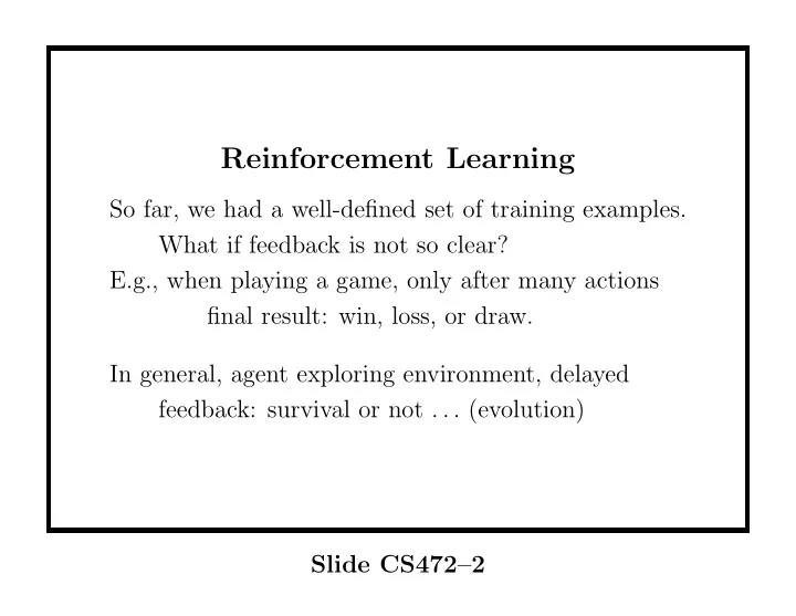
Reinforcement Learning So far, we had a well-defined set of training examples. What if feedback is not so clear? E.g., when playing a game, only after many actions final result: win, loss, or draw. In general, agent exploring environment, delayed feedback: survival or not . . . (evolution) Slide CS472–2

Issue: delayed rewards / feedback . Field: reinforcement learing Main success: Tesauro’s backgammon player (TD Gammon). start from random play; millions of games world-level performance (changed game itself) Chapter 20 R& N. Slide CS472–3

Imagine agent wandering around in environment. How does it learn utility values of each state? (i.e., what are good / bad states? avoid bad ones...) Reinforcement learning will tell us how! Slide CS472–4

Compare: in backgammon game: states = boards. only clear feedback in final states (win/loss). We want to know utility of the other states Intuitively: utility = chance of winning. At first, we only know this for the end states. Reinforcement learning: computes for intermediate states. Play by moving to maximum utility states! back to simplified world . . . Slide CS472–5

3 + 1 2 − 1 START 1 Slide CS472–7 1 2 3 4

.5 .5 .33 1.0 +1 3 + 1 3 −0.0380 0.0886 0.2152 + 1 .5 .33 .5 .5 .33 .33 1.0 .33 2 2 −0.1646 −0.4430 − 1 −1 − 1 .5 .5 .33 .33 .5 .5 .5 .33 START 1 1 −0.2911 −0.0380 −0.5443 −0.7722 .5 .33 .5 1 2 3 4 1 2 3 4 (a) (b) (c) Slide CS472–8

Example of passive learning in a known environment . Agent just wanders from state to state. Each transition is made with a fixed probability. Initially: only two known reward positions: State (4,2) — a loss / poison / reward − 1 (utility) State (4,3) — a win / food / reward +1 (utility) How does the agent learn about the utility, i.e., expected value , of the other states? Slide CS472–9

Three strategies: (a) “Sampling” (Naive updating) (b) “Calculation” / “Equation solving” (Adaptive dynamic programming) (c) “in between (a) and (b)” (Temporal Difference Learning — TD learning) used for backgammon Slide CS472–10

Naive updating (a) “Sampling” — agent makes random runs through environment; collect statistics on final payoff for each state (e.g. when at (2,3), how often do you reach +1 vs. − 1?) Learning algorithm keeps a running average for each state. Provably converges to true expected values (utilities). Slide CS472–11

Main drawback: slow convergence . See next figure. In relatively small world takes agent over 1000 sequences to get a reasonably small ( < 0 . 1) root-mean-square error compared with true expected values. Slide CS472–12

1 (4,3) 0.5 Utility estimates (3,3) 0 (2,3) (1,1) -0.5 (3,1) (4,1) -1 (4,2) 0 200 400 600 800 1000 Number of epochs Slide CS472–14

0.6 0.5 RMS error in utility 0.4 0.3 0.2 0.1 0 0 200 400 600 800 1000 Number of epochs Slide CS472–16

Question: Is sampling necessary? Can we do something completely different? Note: agent knows the environment (i.e. probability of state transitions) and final rewards. Slide CS472–17

Upon, refection we note that the utilities must be completely defined by what the agent already knows about the environment. Slide CS472–18

Adaptive dynamic programming Some intuition first. Consider U (3 , 3) From figure we see that U (3 , 3) = 0 . 33 × U (4 , 3) + 0 . 33 × U (2 , 3) + 0 . 33 × U (3 , 2) = 0 . 33 × 1 . 0 + 0 . 33 × 0 . 0886 + 0 . 33 × − 0 . 4430 = 0 . 2152 Check e.g. U (3 , 1) yourself. Slide CS472–19

Utilities follow basic laws of probabilities: write down equations; solve for unknowns. Utilities follow from: U ( i ) = R ( i ) + j M i,j U ( j ) ( ⋆ ) � (note: i, j over states.) R ( i ) is the reward associated with being in state i . (often non-zero for only a few end states) M i,j is the probability of transition from state i to j . Slide CS472–20

Dynamic programming style methods can be used to solve the set of equations. Major drawback: number of equations and number of unknowns. E.g. for backgammon: roughly 10 50 equations with 10 50 unknowns. Infeasibly large. Slide CS472–21

Temporal difference learning combine “sampling” with “calculation” or stated differently: it’s using a sampling approach to solve the set of equations. Consider the transitions, observed by a wandering agent. Use an observed transition to adjust the utilities of the observed states to bring them closer to the constraint equations. Slide CS472–22

Temporal difference learning When observing a transition from i to j , bring U ( i ) value closer to that of U ( j ) Use update rule: U ( i ) ← U ( i ) + α ( R ( i ) + U ( j ) − U ( i )) ( ⋆⋆ ) α is the learning rate parameter rule is called the temporal-difference or TD equation. (note we take the difference between successive states.) Slide CS472–23

At first blush, the rule: U ( i ) ← U ( i ) + α ( R ( i ) + U ( j ) − U ( i )) ( ⋆⋆ ) may appear to be a bad way to solve/approximate: U ( i ) = R ( i ) + j M i,j U ( j ) ( ⋆ ) � Note that ( ⋆⋆ ) brings U ( i ) closer to U ( j ) but in ( ⋆ ) we really want the weighted average over the neighboring states! Issue resolves itself, because over time, we sample from the transitions out of i . So, successive applications of ( ⋆⋆ ) average over neighboring states. (keep α appropriately small) Slide CS472–24

Performance Runs noisier than Naive Updating (averaging), but smaller error. In our 4x3 world, we get a root-mean-square error of less than 0.07 after 1000 examples. Also, note that compared to Adaptive Dynamic Programming we only deal with observed states during sample runs. I.e., in backgammon consider only a few hundreds of thousands of states out of 10 50 . Represent utility function implicitly (no table) in neural network. Slide CS472–25

1 (4,3) 0.5 Utility estimates (3,3) (2,3) 0 (1,1) -0.5 (3,1) (4,1) -1 (4,2) 0 200 400 600 800 1000 Number of epochs Slide CS472–27

0.6 0.5 RMS error in utility 0.4 0.3 0.2 0.1 0 0 200 400 600 800 1000 Number of epochs Slide CS472–29

Reinforcement learning is a very rich domain of study. In some sense, touches on much of the core of AI. “How does an agent learn to take the right actions in its environment” In general, pick action that leads to state with highest utility as learned so far. Slide CS472–30

E.g. in backgammon pick legal move leading to state with highest expected payoff (chance of winning). Initially moves random. But TD rule starts learning from winning and losing games, by moving utility values backwards. (states leading to lost positions start getting low utility after a series of TD rule applications; states leading to wins see there utilities rise slowly.) Slide CS472–31

Extensions — Active learning — exploration. now and then make new (non utility optimizing move) see n - armed bandit problem p. 611 R&N. — learning action-value functions Q ( a, i ) denotes value of taking action a in state i we have: U ( i ) = max a Q ( a, i ) Slide CS472–32

— generalization in reinforcement learning use implicit representation of utility function e.g. a neural network as in backgammon. input nodes encode board position activation of output node gives utility — genetic algorithms — feedback: fitness done in search part. Slide CS472–33